

172
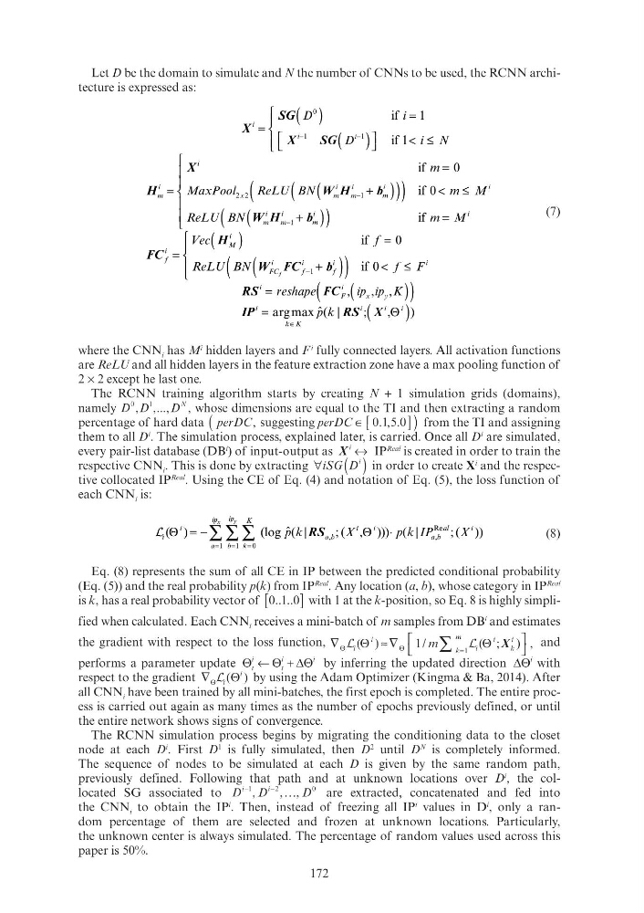
Let D be the domain to simulate and N the number of CNNs to be used, the RCNN architecture is expressed as:
( )
(
)
(
)
(
)
(
)
(
)
( )
(
)
(
)
(
)
(
)
0
if
1
if 1
if
0
if
0
arg ma
f
i
i
i
i
i
i
i
(
)
(
)
(
) if
m
x
mm
m
(
(
(
2 2
1
2
(
(
(
i
i
i
i
))
if
m
m
m
1
i
M
i
f
i
i
i
i
)) if
f
f
1
FC f
i
i
( F x y
(
i
D
i
)
0
if
i N
if 1
m M
))) 0
i
i
i
i
i
i
(
)
(
)
(
) if 0
x
m
m
m
2 2
1
2
(
(
(
ReLU BN
m M
(
)
(
)
i
))
if
m
m
m
1
Vec
f
( )
if
i
M
ReLU BN
f F
(
)
(
) 0
i
i
i
)) if 0
FC
f
f
1
f
reshape
ip ip K
(
(
,
i
( F x y
x
(
,
, , ,
(
⎧
⎪
⎧ ⎧
= ⎨
⎪ ⎪
⎡
⎤
( )
1
1
(
i 1
( )
1
(
i i
⎪
⎨ ⎨
⎣
⎦
( )
D )
( ( ( D )
1
i
⎡ ⎡
⎩ ⎪ ⎪
⎧
⎪
⎧ ⎧
⎪
⎪ ⎪
m m
))) if 0
i
))) if 0
m
⎪
⎪
⎪ ⎪
m
))
if
i
))
if
m
⎩
⎪ ⎪
⎧
⎪
⎧ ⎧
= ⎨
⎪ ⎪
f f
)) if 0
i
)) if 0
f
⎪
⎨ ⎨
⎩
⎪ ⎪
=
SG
X
i 1 1
i 1
X
x
m
m
m
2 2
1
2
(
(
(
H
i
m
i
i
i
i
(
(
(
MaxPool
ReLU BN (
(
(
2 2
1
(
(
(
i
i
i
i
(
(
(
x
m
m
m
2 2
1
2
(
(
(
=
W
i
i i
1
i
i i
m
m
m
m 1
m
FC
i
i i
FC
f
f
f 1
f
RS
i
reshape ( (
=
IP
(
)
x ( |
)
(
)
ˆ
(
i
i
i
( (
k K
( (
( ( (
(7)
where the CNN i has M
i hidden layers and F
i fully connected layers. All activation functions
are ReLU and all hidden layers in the feature extraction zone have a max pooling function of
2 × 2 except he last one.
The RCNN training algorithm starts by creating N + 1 simulation grids (domains),
namely D D
D
N
0
1
D
, ,
D ..., , whose dimensions are equal to the TI and then extracting a random
percentage of hard data perDC
p erDC
perDC
i
∈ [
]
. , .
(
)
. .
from the TI and assigning
them to all D
i . The simulation process, explained later, is carried. Once all D
i are simulated,
every pair-list database (DB
i ) of input-output as X
i ↔ IP
Real is created in order to train the
respective CNN i . This is done by extracting ∀
( )
iSG D
(
i
in order to create X
i and the respective collocated IP
Real . Using the CE of Eq. (4) and notation of Eq. (5), the loss function of
each CNN i is:
,
,
0
(
))
y
x
ip
ip
K
i
i
i
a l
i
Re
(l ˆ
)
; (
; (
a b
a b
,
,
( g
i ( )
a
b
k
1
1 1
( |
;(
( |
;(
e
i
( |
(
))) ( |
; (
))) ( |
( |
;(
Re
,
,
( |
;(
,
, ))) ( |
( | ,
1
1 1
(log (log (log
X
; (
))) )))
i
; (
)))
( |
( ( |
( ( |
;(
(
, )))
= −
( )
( )
( )
∑ ∑ ∑
∑ ∑ ∑
L i i
(8)
Eq. (8) represents the sum of all CE in IP between the predicted conditional probability
(Eq. (5)) and the real probability p(k) from IP
Real . Any location (a, b), whose category in IP
Real
is k, has a real probability vector of [
]
0 1 0
.. .. with 1 at the k-position, so Eq. 8 is highly simplified when calculated. Each CNN i receives a mini-batch of m samples from DB
i and estimates
the gradient with respect to the loss function, ∇
≈∇ ⎡
⎣
⎤
⎦
⎤ ⎤
=
∑
Θ
Θ
⎣
≈ ∇ ⎡
Θ
≈ ∇
≈ ∇ ⎡
⎣
⎡ ⎡
Θ
≈ ∇
i
i
i
k
i
k
m
(
)
k
i
/ ∑ L
∑ ∑ i
L L
k
m
(Θ
i
,
1
and
performs a parameter update Θ
Θ ΔΘ
t
i
t
i
i
ΔΘ
+
Θ t
i
by inferring the updated direction ΔΘ
i with
respect to the gradient ∇ Θ L i
L L
i
( )
Θ
i
by using the Adam Optimizer (Kingma & Ba, 2014). After
all CNN i have been trained by all mini-batches, the first epoch is completed. The entire process is carried out again as many times as the number of epochs previously defined, or until
the entire network shows signs of convergence.
The RCNN simulation process begins by migrating the conditioning data to the closet
node at each D
i . First D
1 is fully simulated, then D
2 until D
N is completely informed.
The sequence of nodes to be simulated at each D is given by the same random path,
previously defined. Following that path and at unknown locations over D
i , the collocated SG associated to D D
D
i
i
D
1
2
i
D
−
i
D
0
,
,
D
,
…
are extracted, concatenated and fed into
the CNN i to obtain the IP
i . Then, instead of freezing all IP
i values in D
i , only a random percentage of them are selected and frozen at unknown locations. Particularly,
the unknown center is always simulated. The percentage of random values used across this
paper is 50%.
Let D be the domain to simulate and N the number of CNNs to be used, the RCNN architecture is expressed as:
( )
(
)
(
)
(
)
(
)
(
)
( )
(
)
(
)
(
)
(
)
0
if
1
if 1
if
0
if
0
arg ma
f
i
i
i
i
i
i
i
(
)
(
)
(
) if
m
x
mm
m
(
(
(
2 2
1
2
(
(
(
i
i
i
i
))
if
m
m
m
1
i
M
i
f
i
i
i
i
)) if
f
f
1
FC f
i
i
( F x y
(
i
D
i
)
0
if
i N
if 1
m M
))) 0
i
i
i
i
i
i
(
)
(
)
(
) if 0
x
m
m
m
2 2
1
2
(
(
(
ReLU BN
m M
(
)
(
)
i
))
if
m
m
m
1
Vec
f
( )
if
i
M
ReLU BN
f F
(
)
(
) 0
i
i
i
)) if 0
FC
f
f
1
f
reshape
ip ip K
(
(
,
i
( F x y
x
(
,
, , ,
(
⎧
⎪
⎧ ⎧
= ⎨
⎪ ⎪
⎡
⎤
( )
1
1
(
i 1
( )
1
(
i i
⎪
⎨ ⎨
⎣
⎦
( )
D )
( ( ( D )
1
i
⎡ ⎡
⎩ ⎪ ⎪
⎧
⎪
⎧ ⎧
⎪
⎪ ⎪
m m
))) if 0
i
))) if 0
m
⎪
⎪
⎪ ⎪
m
))
if
i
))
if
m
⎩
⎪ ⎪
⎧
⎪
⎧ ⎧
= ⎨
⎪ ⎪
f f
)) if 0
i
)) if 0
f
⎪
⎨ ⎨
⎩
⎪ ⎪
=
SG
X
i 1 1
i 1
X
x
m
m
m
2 2
1
2
(
(
(
H
i
m
i
i
i
i
(
(
(
MaxPool
ReLU BN (
(
(
2 2
1
(
(
(
i
i
i
i
(
(
(
x
m
m
m
2 2
1
2
(
(
(
=
W
i
i i
1
i
i i
m
m
m
m 1
m
FC
i
i i
FC
f
f
f 1
f
RS
i
reshape ( (
=
IP
(
)
x ( |
)
(
)
ˆ
(
i
i
i
( (
k K
( (
( ( (
(7)
where the CNN i has M
i hidden layers and F
i fully connected layers. All activation functions
are ReLU and all hidden layers in the feature extraction zone have a max pooling function of
2 × 2 except he last one.
The RCNN training algorithm starts by creating N + 1 simulation grids (domains),
namely D D
D
N
0
1
D
, ,
D ..., , whose dimensions are equal to the TI and then extracting a random
percentage of hard data perDC
p erDC
perDC
i
∈ [
]
. , .
(
)
. .
from the TI and assigning
them to all D
i . The simulation process, explained later, is carried. Once all D
i are simulated,
every pair-list database (DB
i ) of input-output as X
i ↔ IP
Real is created in order to train the
respective CNN i . This is done by extracting ∀
( )
iSG D
(
i
in order to create X
i and the respective collocated IP
Real . Using the CE of Eq. (4) and notation of Eq. (5), the loss function of
each CNN i is:
,
,
0
(
))
y
x
ip
ip
K
i
i
i
a l
i
Re
(l ˆ
)
; (
; (
a b
a b
,
,
( g
i ( )
a
b
k
1
1 1
( |
;(
( |
;(
e
i
( |
(
))) ( |
; (
))) ( |
( |
;(
Re
,
,
( |
;(
,
, ))) ( |
( | ,
1
1 1
(log (log (log
X
; (
))) )))
i
; (
)))
( |
( ( |
( ( |
;(
(
, )))
= −
( )
( )
( )
∑ ∑ ∑
∑ ∑ ∑
L i i
(8)
Eq. (8) represents the sum of all CE in IP between the predicted conditional probability
(Eq. (5)) and the real probability p(k) from IP
Real . Any location (a, b), whose category in IP
Real
is k, has a real probability vector of [
]
0 1 0
.. .. with 1 at the k-position, so Eq. 8 is highly simplified when calculated. Each CNN i receives a mini-batch of m samples from DB
i and estimates
the gradient with respect to the loss function, ∇
≈∇ ⎡
⎣
⎤
⎦
⎤ ⎤
=
∑
Θ
Θ
⎣
≈ ∇ ⎡
Θ
≈ ∇
≈ ∇ ⎡
⎣
⎡ ⎡
Θ
≈ ∇
i
i
i
k
i
k
m
(
)
k
i
/ ∑ L
∑ ∑ i
L L
k
m
(Θ
i
,
1
and
performs a parameter update Θ
Θ ΔΘ
t
i
t
i
i
ΔΘ
+
Θ t
i
by inferring the updated direction ΔΘ
i with
respect to the gradient ∇ Θ L i
L L
i
( )
Θ
i
by using the Adam Optimizer (Kingma & Ba, 2014). After
all CNN i have been trained by all mini-batches, the first epoch is completed. The entire process is carried out again as many times as the number of epochs previously defined, or until
the entire network shows signs of convergence.
The RCNN simulation process begins by migrating the conditioning data to the closet
node at each D
i . First D
1 is fully simulated, then D
2 until D
N is completely informed.
The sequence of nodes to be simulated at each D is given by the same random path,
previously defined. Following that path and at unknown locations over D
i , the collocated SG associated to D D
D
i
i
D
1
2
i
D
−
i
D
0
,
,
D
,
…
are extracted, concatenated and fed into
the CNN i to obtain the IP
i . Then, instead of freezing all IP
i values in D
i , only a random percentage of them are selected and frozen at unknown locations. Particularly,
the unknown center is always simulated. The percentage of random values used across this
paper is 50%.