

171
(CE), and for continuous values the Mean Squared Error (MSE) between each predicted
value ˆ k
y and the real one y k :
( )
( )
(
) ( )
( )
2
1
1
)
ˆ
K
P
1
k
k
k
k
1
y
(
CE ( )
: ( )
( k
P
1
( (
∑
∑
( )
(
) ( )
( )
p
p
p
p
( )
(
) ( )
( )
g g ( )
(
) ( )
( ) P
∑
∑
( )
(
) ( )
( )
1
ˆ ( )) ( )
( )
1
l
( ( )) ( )
( )
1
( )
( )
1
( ) )
g ( )
(
) ( )
l
( ( )) ( )
log
:
( )
(
) ( )
( )) ( )
(4)
3 THE RECURSIVE CONVOLUTIONAL NEURAL NETWORK APPROACH
Let SG ( , , )
sg
x
y
,sg
and IP ( , , )
ip
x
y
, ip
be the search grid and inner pattern, whose dimensions
sg sg ip
x
y
g x
, ,
sg y
sg
and ip y are odd positive integers to ensure the existence of a collocated center
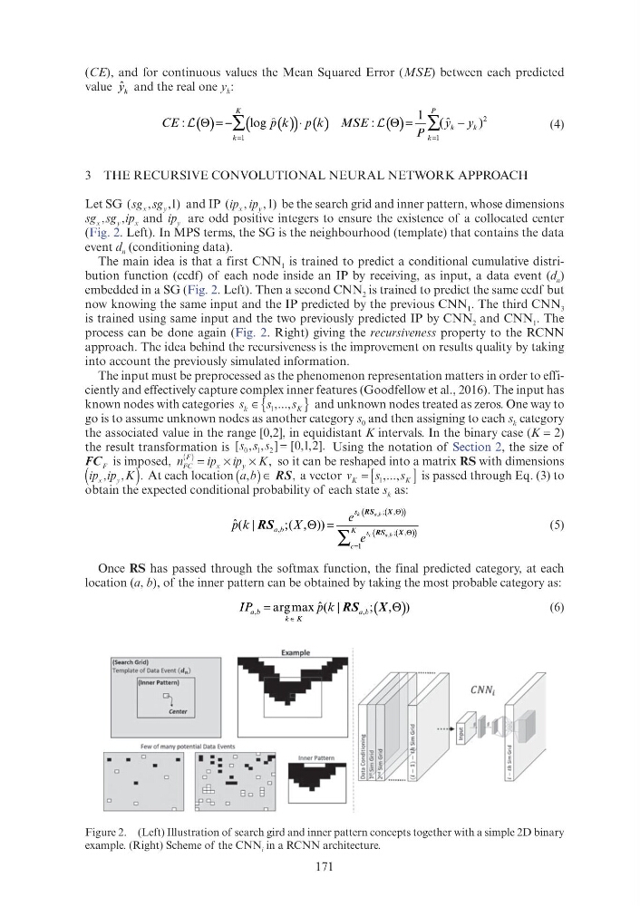
(Fig. 2. Left). In MPS terms, the SG is the neighbourhood (template) that contains the data
event d n (conditioning data).
The main idea is that a first CNN 1 is trained to predict a conditional cumulative distribution function (ccdf) of each node inside an IP by receiving, as input, a data event (d n )
embedded in a SG (Fig. 2. Left). Then a second CNN 2 is trained to predict the same ccdf but
now knowing the same input and the IP predicted by the previous CNN 1 . The third CNN 3
is trained using same input and the two previously predicted IP by CNN 2 and CNN 1 . The
process can be done again (Fig. 2. Right) giving the recursiveness property to the RCNN
approach. The idea behind the recursiveness is the improvement on results quality by taking
into account the previously simulated information.
The input must be preprocessed as the phenomenon representation matters in order to efficiently and effectively capture complex inner features (Goodfellow et al., 2016). The input has
known nodes with categories s k ∈{
}
s
s K
s
s and unknown nodes treated as zeros. One way to
go is to assume unknown nodes as another category s 0 and then assigning to each s k category
the associated value in the range [0,2], in equidistant K intervals. In the binary case (K = 2)
the result transformation is [ , , ] [ , , ].
s
,
0 1
,s , 2
0 1
, 2
=
Using the notation of Section 2, the size of
FC F is imposed, n
ip i
i
p K
i
FC
x
y
ip i
( )
F
ip i
, so it can be reshaped into a matrix RS with dimensions
ip ip K
x
y
p
, ,
ip y
ip
.
(
)
p
At each location
,
( )
y
a b
,b ∈ RS a vector v K [
]
s
s K
s
s is passed through Eq. (3) to
obtain the expected conditional probability of each state s k as:
( )
(
)
( )
(
)
,
,
; ,
(
,
; ,
(
1
( |
;( , )
ˆ
k
a b
( ,
c
ab
( ,
s
a b
,
K s
c
e
p k
( |
;(
|
;(
ˆ
,
e
Θ
Θ
=
=
) ∑
RS
X
(
;(
a b
RS
X
(
;(
a b
(5)
Once RS has passed through the softmax function, the final predicted category, at each
location (a, b), of the inner pattern can be obtained by taking the most probable category as:
( )
,
,
ˆ( |
; , )
( )
a b
a b
,
,
|
,
k K
IP
(
ˆ
a b
,
g
(
; ,
(
| |
arg max ( (
ˆ
arg max ( (
(
; ; (
(6)
Figure 2. (Left) Illustration of search gird and inner pattern concepts together with a simple 2D binary
example. (Right) Scheme of the CNN i in a RCNN architecture.
(Search Grid}
Template of Data Event (d , )
(Inner Pattern}
Center
CJ
I • •
CJ
Inner Pattern
.. CJ ..
~
CJ •
CJ
CJ
CJ
EEb
CJ
8CJ El
q,
CJ
(CE), and for continuous values the Mean Squared Error (MSE) between each predicted
value ˆ k
y and the real one y k :
( )
( )
(
) ( )
( )
2
1
1
)
ˆ
K
P
1
k
k
k
k
1
y
(
CE ( )
: ( )
( k
P
1
( (
∑
∑
( )
(
) ( )
( )
p
p
p
p
( )
(
) ( )
( )
g g ( )
(
) ( )
( ) P
∑
∑
( )
(
) ( )
( )
1
ˆ ( )) ( )
( )
1
l
( ( )) ( )
( )
1
( )
( )
1
( ) )
g ( )
(
) ( )
l
( ( )) ( )
log
:
( )
(
) ( )
( )) ( )
(4)
3 THE RECURSIVE CONVOLUTIONAL NEURAL NETWORK APPROACH
Let SG ( , , )
sg
x
y
,sg
and IP ( , , )
ip
x
y
, ip
be the search grid and inner pattern, whose dimensions
sg sg ip
x
y
g x
, ,
sg y
sg
and ip y are odd positive integers to ensure the existence of a collocated center
(Fig. 2. Left). In MPS terms, the SG is the neighbourhood (template) that contains the data
event d n (conditioning data).
The main idea is that a first CNN 1 is trained to predict a conditional cumulative distribution function (ccdf) of each node inside an IP by receiving, as input, a data event (d n )
embedded in a SG (Fig. 2. Left). Then a second CNN 2 is trained to predict the same ccdf but
now knowing the same input and the IP predicted by the previous CNN 1 . The third CNN 3
is trained using same input and the two previously predicted IP by CNN 2 and CNN 1 . The
process can be done again (Fig. 2. Right) giving the recursiveness property to the RCNN
approach. The idea behind the recursiveness is the improvement on results quality by taking
into account the previously simulated information.
The input must be preprocessed as the phenomenon representation matters in order to efficiently and effectively capture complex inner features (Goodfellow et al., 2016). The input has
known nodes with categories s k ∈{
}
s
s K
s
s and unknown nodes treated as zeros. One way to
go is to assume unknown nodes as another category s 0 and then assigning to each s k category
the associated value in the range [0,2], in equidistant K intervals. In the binary case (K = 2)
the result transformation is [ , , ] [ , , ].
s
,
0 1
,s , 2
0 1
, 2
=
Using the notation of Section 2, the size of
FC F is imposed, n
ip i
i
p K
i
FC
x
y
ip i
( )
F
ip i
, so it can be reshaped into a matrix RS with dimensions
ip ip K
x
y
p
, ,
ip y
ip
.
(
)
p
At each location
,
( )
y
a b
,b ∈ RS a vector v K [
]
s
s K
s
s is passed through Eq. (3) to
obtain the expected conditional probability of each state s k as:
( )
(
)
( )
(
)
,
,
; ,
(
,
; ,
(
1
( |
;( , )
ˆ
k
a b
( ,
c
ab
( ,
s
a b
,
K s
c
e
p k
( |
;(
|
;(
ˆ
,
e
Θ
Θ
=
=
) ∑
RS
X
(
;(
a b
RS
X
(
;(
a b
(5)
Once RS has passed through the softmax function, the final predicted category, at each
location (a, b), of the inner pattern can be obtained by taking the most probable category as:
( )
,
,
ˆ( |
; , )
( )
a b
a b
,
,
|
,
k K
IP
(
ˆ
a b
,
g
(
; ,
(
| |
arg max ( (
ˆ
arg max ( (
(
; ; (
(6)
Figure 2. (Left) Illustration of search gird and inner pattern concepts together with a simple 2D binary
example. (Right) Scheme of the CNN i in a RCNN architecture.
(Search Grid}
Template of Data Event (d , )
(Inner Pattern}
Center
CJ
I • •
CJ
Inner Pattern
.. CJ ..
~
CJ •
CJ
CJ
CJ
EEb
CJ
8CJ El
q,
CJ