

138
this ratio is approximately constant at 1.77, which is the square root of π. Theory shows that
for bigaussian data, this relationship holds true and this result shows that the normal score
transformation of Nb 2 O 5 is approximately bigaussian.
The next step is to perform a Gaussian anamorphosis, calculating the normal scores values
of the grades and fit a set of Hermite polynomials to describe the relationship between the
sample grades and their corresponding normal scores values. Hansmann (2016) says that
the number of Hermite coefficient used to fit the anamorphosis model, can vary, and the
optimum number depends on how well the polynomial set fits the underlying distribution. It
is recommended to use less than 100 coefficients, although in this study 30 coefficients were
sufficient, see Figure 5.
6 VARIOGRAPHIC ANALYSIS
Two different variographic analysis were performed to carry out the estimation for both
approaches.
Summing up, there are two important differences:
• First, for multivariate LUC (MLUC) a variogram model of the raw grades was used.
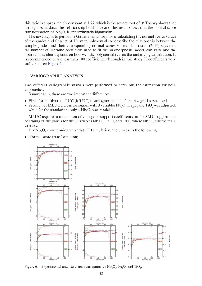
• Second, for MLUC a cross variogram with 3 variables Nb 2 O 5 , Fe 2 O 3 and TiO 2 was adjusted,
while for the simulation, only a Nb 2 O 5 was modeled.
MLUC requires a calculation of change of support coefficients on the SMU support and
cokriging of the panels for the 3 variables Nb 2 O 5 , Fe 2 O 3 and TiO 2 , where Nb 2 O 5 was the main
variable.
For Nb 2 O 5 conditioning univariate TB simulation, the process is the following:
• Normal score transformation;
Figure 6. Experimental and fitted cross variogram for Nb 2 O 5 , Fe 2 O 3 and TiO 2 .
'
•
· '
:
Diatance(a)
ni;o~e(•~so
Diatance(a)
ni;o~e
rr
1 \\~c
Dia Um<:e (a)
NllO
N200
D-90
N200
: 9Jl 0
~
~·
I
0
N200 0
0 0
Dht.ance <•I
Oiatance <•iso
'"
,-~;;. .,;···'"·
, 5
F
o _ _;:;c__ '' ..:; ·;~ ::_'_'-' ":s ;::. o_--F'----,
/'"r
D-90
s
D-90
- - - - - - - - - - - - - - - - - - - 1.5
,}t
NllO
' ' \ •. ..
N200 fs
N200
Diat.anc" <•I
this ratio is approximately constant at 1.77, which is the square root of π. Theory shows that
for bigaussian data, this relationship holds true and this result shows that the normal score
transformation of Nb 2 O 5 is approximately bigaussian.
The next step is to perform a Gaussian anamorphosis, calculating the normal scores values
of the grades and fit a set of Hermite polynomials to describe the relationship between the
sample grades and their corresponding normal scores values. Hansmann (2016) says that
the number of Hermite coefficient used to fit the anamorphosis model, can vary, and the
optimum number depends on how well the polynomial set fits the underlying distribution. It
is recommended to use less than 100 coefficients, although in this study 30 coefficients were
sufficient, see Figure 5.
6 VARIOGRAPHIC ANALYSIS
Two different variographic analysis were performed to carry out the estimation for both
approaches.
Summing up, there are two important differences:
• First, for multivariate LUC (MLUC) a variogram model of the raw grades was used.
• Second, for MLUC a cross variogram with 3 variables Nb 2 O 5 , Fe 2 O 3 and TiO 2 was adjusted,
while for the simulation, only a Nb 2 O 5 was modeled.
MLUC requires a calculation of change of support coefficients on the SMU support and
cokriging of the panels for the 3 variables Nb 2 O 5 , Fe 2 O 3 and TiO 2 , where Nb 2 O 5 was the main
variable.
For Nb 2 O 5 conditioning univariate TB simulation, the process is the following:
• Normal score transformation;
Figure 6. Experimental and fitted cross variogram for Nb 2 O 5 , Fe 2 O 3 and TiO 2 .
'
•
· '
:
Diatance(a)
ni;o~e(•~so
Diatance(a)
ni;o~e
rr
1 \\~c
Dia Um<:e (a)
NllO
N200
D-90
N200
: 9Jl 0
~
~·
I
0
N200 0
0 0
Dht.ance <•I
Oiatance <•iso
'"
,-~;;. .,;···'"·
, 5
F
o _ _;:;c__ '' ..:; ·;~ ::_'_'-' ":s ;::. o_--F'----,
/'"r
D-90
s
D-90
- - - - - - - - - - - - - - - - - - - 1.5
,}t
NllO
' ' \ •. ..
N200 fs
N200
Diat.anc" <•I