

118
1. Estimate metal grade in large panels representing monthly or quarterly production. Only
data located in or very close to the panels are used to estimate the grade of the panels by
kriging.
2. Calculate uncertainty on the estimated panel grade. As shown in formula (1) the uncertainty is calculated from kriging variance (OKVar), declustered variance of the data used
for the estimation (VarDat), and the estimated grade (EstGr).
The kriging variance is based on a variogram model standardized to sill of 1.0. To calculate
the uncertainty on the estimated panel grade the kriging variance is adjusted for local variability by a squared coefficient of variation (VarDat/EstGr
2
). If a panel represents monthly
production, uncertainty on the estimated panels within one year period can be calculated as
follows:
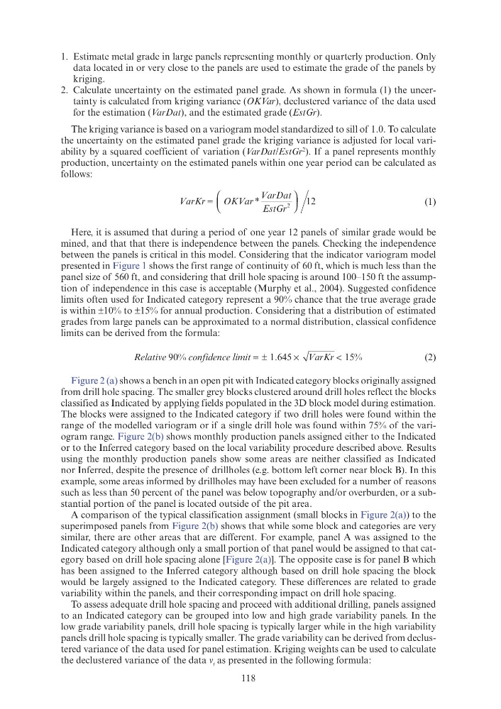
VarKr
O
K K
KVar
VarDat
EstGr
⎛
⎝ ⎝ ⎝
⎞
⎠
⎞ ⎞ ⎞ ⎞
⎠ ⎠
⎞ ⎞ ⎞ ⎞
*
2
12
(1)
Here, it is assumed that during a period of one year 12 panels of similar grade would be
mined, and that that there is independence between the panels. Checking the independence
between the panels is critical in this model. Considering that the indicator variogram model
presented in Figure 1 shows the first range of continuity of 60 ft, which is much less than the
panel size of 560 ft, and considering that drill hole spacing is around 100–150 ft the assumption of independence in this case is acceptable (Murphy et al., 2004). Suggested confidence
limits often used for Indicated category represent a 90% chance that the true average grade
is within ±10% to ±15% for annual production. Considering that a distribution of estimated
grades from large panels can be approximated to a normal distribution, classical confidence
limits can be derived from the formula:
Relative
confidence l
VarK
90
1 645
15
%
.
confidence limit
1
%
×
<
VarKr K K
(2)
Figure 2 (a) shows a bench in an open pit with Indicated category blocks originally assigned
from drill hole spacing. The smaller grey blocks clustered around drill holes reflect the blocks
classified as Indicated by applying fields populated in the 3D block model during estimation.
The blocks were assigned to the Indicated category if two drill holes were found within the
range of the modelled variogram or if a single drill hole was found within 75% of the variogram range. Figure 2(b) shows monthly production panels assigned either to the Indicated
or to the Inferred category based on the local variability procedure described above. Results
using the monthly production panels show some areas are neither classified as Indicated
nor Inferred, despite the presence of drillholes (e.g. bottom left corner near block B). In this
example, some areas informed by drillholes may have been excluded for a number of reasons
such as less than 50 percent of the panel was below topography and/or overburden, or a substantial portion of the panel is located outside of the pit area.
A comparison of the typical classification assignment (small blocks in Figure 2(a)) to the
superimposed panels from Figure 2(b) shows that while some block and categories are very
similar, there are other areas that are different. For example, panel A was assigned to the
Indicated category although only a small portion of that panel would be assigned to that category based on drill hole spacing alone [Figure 2(a)]. The opposite case is for panel B which
has been assigned to the Inferred category although based on drill hole spacing the block
would be largely assigned to the Indicated category. These differences are related to grade
variability within the panels, and their corresponding impact on drill hole spacing.
To assess adequate drill hole spacing and proceed with additional drilling, panels assigned
to an Indicated category can be grouped into low and high grade variability panels. In the
low grade variability panels, drill hole spacing is typically larger while in the high variability
panels drill hole spacing is typically smaller. The grade variability can be derived from declustered variance of the data used for panel estimation. Kriging weights can be used to calculate
the declustered variance of the data v i as presented in the following formula:
1. Estimate metal grade in large panels representing monthly or quarterly production. Only
data located in or very close to the panels are used to estimate the grade of the panels by
kriging.
2. Calculate uncertainty on the estimated panel grade. As shown in formula (1) the uncertainty is calculated from kriging variance (OKVar), declustered variance of the data used
for the estimation (VarDat), and the estimated grade (EstGr).
The kriging variance is based on a variogram model standardized to sill of 1.0. To calculate
the uncertainty on the estimated panel grade the kriging variance is adjusted for local variability by a squared coefficient of variation (VarDat/EstGr
2
). If a panel represents monthly
production, uncertainty on the estimated panels within one year period can be calculated as
follows:
VarKr
O
K K
KVar
VarDat
EstGr
⎛
⎝ ⎝ ⎝
⎞
⎠
⎞ ⎞ ⎞ ⎞
⎠ ⎠
⎞ ⎞ ⎞ ⎞
*
2
12
(1)
Here, it is assumed that during a period of one year 12 panels of similar grade would be
mined, and that that there is independence between the panels. Checking the independence
between the panels is critical in this model. Considering that the indicator variogram model
presented in Figure 1 shows the first range of continuity of 60 ft, which is much less than the
panel size of 560 ft, and considering that drill hole spacing is around 100–150 ft the assumption of independence in this case is acceptable (Murphy et al., 2004). Suggested confidence
limits often used for Indicated category represent a 90% chance that the true average grade
is within ±10% to ±15% for annual production. Considering that a distribution of estimated
grades from large panels can be approximated to a normal distribution, classical confidence
limits can be derived from the formula:
Relative
confidence l
VarK
90
1 645
15
%
.
confidence limit
1
%
×
<
VarKr K K
(2)
Figure 2 (a) shows a bench in an open pit with Indicated category blocks originally assigned
from drill hole spacing. The smaller grey blocks clustered around drill holes reflect the blocks
classified as Indicated by applying fields populated in the 3D block model during estimation.
The blocks were assigned to the Indicated category if two drill holes were found within the
range of the modelled variogram or if a single drill hole was found within 75% of the variogram range. Figure 2(b) shows monthly production panels assigned either to the Indicated
or to the Inferred category based on the local variability procedure described above. Results
using the monthly production panels show some areas are neither classified as Indicated
nor Inferred, despite the presence of drillholes (e.g. bottom left corner near block B). In this
example, some areas informed by drillholes may have been excluded for a number of reasons
such as less than 50 percent of the panel was below topography and/or overburden, or a substantial portion of the panel is located outside of the pit area.
A comparison of the typical classification assignment (small blocks in Figure 2(a)) to the
superimposed panels from Figure 2(b) shows that while some block and categories are very
similar, there are other areas that are different. For example, panel A was assigned to the
Indicated category although only a small portion of that panel would be assigned to that category based on drill hole spacing alone [Figure 2(a)]. The opposite case is for panel B which
has been assigned to the Inferred category although based on drill hole spacing the block
would be largely assigned to the Indicated category. These differences are related to grade
variability within the panels, and their corresponding impact on drill hole spacing.
To assess adequate drill hole spacing and proceed with additional drilling, panels assigned
to an Indicated category can be grouped into low and high grade variability panels. In the
low grade variability panels, drill hole spacing is typically larger while in the high variability
panels drill hole spacing is typically smaller. The grade variability can be derived from declustered variance of the data used for panel estimation. Kriging weights can be used to calculate
the declustered variance of the data v i as presented in the following formula: