

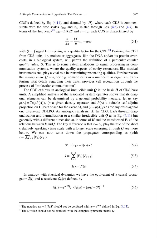
CDS’s defined by Eq. (4.11), and denoted by H
j ⟩, where each CDS is commensurate with the time scales τ corr and τ rel related through Eqs. (4.6) and (4.7). In
terms of the frequency
23
ω 0 = ℏ ̸ k B T and τ = τ rel each CDS is characterized by
n
4π
=
kT
ℏ
τ rel = ω 0 τ
ð5:1Þ
with Q =
R ω 0 τdΩ = n serving as a quality factor for the CDE.
24 Deriving the CDE
from CDS units, i.e. molecular aggregates, like the DNA and/or its protein overcoats, in a biological system, will permit the definition of a particular cellular
quality value, Q. This is to some extent analogous to signal processing in communication systems, where the quality aspects of cavity resonators, like musical
instruments etc., play a vital role in transmitting resonating qualities. For that reason
the quality value Q = n, for e.g. somatic cells in a multicellular organism, transferring vital details regarding their traits, provides cell recognition through the
process of “molecular communication”.
The CDE exhibits an analogical irreducible unit Q in the basis H of CDS base
units. A simplified analysis of the associated system operator shows that its diagonal elements can be determined by a general probability measure, let us say
p A
ð Þ = Tr ρP A
ð Þ
ð
Þ, (ρ a given density operator and P(A) a suitable self-adjoint
projection on Hilbert Space for the event A), and (1 – p(A))p(A) for any off-diagonal
one displaying ODLRO. An analogous analysis, cf. the CDS, leads through diagonalization and thermalization to a similar irreducible unit Q as in Eq. (4.11) but
generally with a different dimension m, in terms of H and the transformed F, cf. the
relations between h and f. The key difference is that τ = τ rel play the role of the short
(relatively speaking) time scale with a longer scale emerging through Q see more
below. We can now write down the propagator corresponding as (with
I = ∑
m
k = 1 F k
j ⟩⟨F k j)
P = ω 0 τ − i
ð
ÞI + iJ
ð5:2Þ
J = ∑
m − 1
k = 1
F k
j ⟩⟨F k + 1 j
ð5:3Þ
H
j ⟩ = F
j ⟩B
ð5:4Þ
In analogy with classical dynamics we have the equivalent of a causal propagator GðtÞ and a resolvent G R ðzÞ defined by
G t
ð Þ = e
− iP
t
τ ; G R ω
ð Þ= ωτI − P
ð
Þ
− 1
ð5:5Þ
23
The notation ω 0 = ℏ ̸ k B T should not be confused with ω = e
iπ ̸ n defined in Eq. (4.13).
24
The Q-value should not be confused with the complex symmetric matrix Q.
A Simple Communication Hypothesis: The Process …
397
j ⟩, where each CDS is commensurate with the time scales τ corr and τ rel related through Eqs. (4.6) and (4.7). In
terms of the frequency
23
ω 0 = ℏ ̸ k B T and τ = τ rel each CDS is characterized by
n
4π
=
kT
ℏ
τ rel = ω 0 τ
ð5:1Þ
with Q =
R ω 0 τdΩ = n serving as a quality factor for the CDE.
24 Deriving the CDE
from CDS units, i.e. molecular aggregates, like the DNA and/or its protein overcoats, in a biological system, will permit the definition of a particular cellular
quality value, Q. This is to some extent analogous to signal processing in communication systems, where the quality aspects of cavity resonators, like musical
instruments etc., play a vital role in transmitting resonating qualities. For that reason
the quality value Q = n, for e.g. somatic cells in a multicellular organism, transferring vital details regarding their traits, provides cell recognition through the
process of “molecular communication”.
The CDE exhibits an analogical irreducible unit Q in the basis H of CDS base
units. A simplified analysis of the associated system operator shows that its diagonal elements can be determined by a general probability measure, let us say
p A
ð Þ = Tr ρP A
ð Þ
ð
Þ, (ρ a given density operator and P(A) a suitable self-adjoint
projection on Hilbert Space for the event A), and (1 – p(A))p(A) for any off-diagonal
one displaying ODLRO. An analogous analysis, cf. the CDS, leads through diagonalization and thermalization to a similar irreducible unit Q as in Eq. (4.11) but
generally with a different dimension m, in terms of H and the transformed F, cf. the
relations between h and f. The key difference is that τ = τ rel play the role of the short
(relatively speaking) time scale with a longer scale emerging through Q see more
below. We can now write down the propagator corresponding as (with
I = ∑
m
k = 1 F k
j ⟩⟨F k j)
P = ω 0 τ − i
ð
ÞI + iJ
ð5:2Þ
J = ∑
m − 1
k = 1
F k
j ⟩⟨F k + 1 j
ð5:3Þ
H
j ⟩ = F
j ⟩B
ð5:4Þ
In analogy with classical dynamics we have the equivalent of a causal propagator GðtÞ and a resolvent G R ðzÞ defined by
G t
ð Þ = e
− iP
t
τ ; G R ω
ð Þ= ωτI − P
ð
Þ
− 1
ð5:5Þ
23
The notation ω 0 = ℏ ̸ k B T should not be confused with ω = e
iπ ̸ n defined in Eq. (4.13).
24
The Q-value should not be confused with the complex symmetric matrix Q.
A Simple Communication Hypothesis: The Process …
397