

Functional Derivatives and Differentiability in Density-Functional Theory
357
where “h.o.” denotes higher-order terms in í µí¼. Therefore, we reach the same conclusion as before: {c i } for Ψ i ∈ is linear in í µí¼ towards the end of variational path.
For those {c i } for Ψ i ∈ , utilizing the additional fact that Ψ i is order-1 strongly
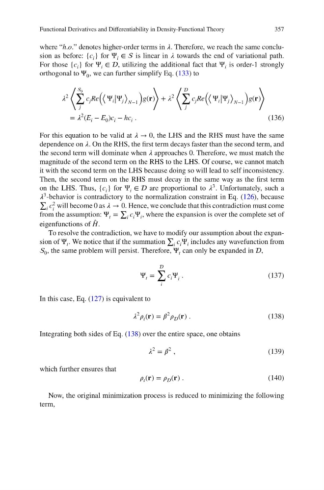
orthogonal to Ψ 0 , we can further simplify Eq. (133) to
í µí¼
2
⟨ 0
∑
j
c j Re
( ⟨ Ψ i |
| Ψ j
⟩
N−1
)
g(í µí°«)
⟩
+ í µí¼
2
⟨
∑
j
c j Re
( ⟨ Ψ i |
| Ψ j
⟩
N−1
)
g(í µí°«)
⟩
= í µí¼
2
(E i − E 0 )c i − hc i .
(136)
For this equation to be valid at í µí¼ → 0, the LHS and the RHS must have the same
dependence on í µí¼. On the RHS, the first term decays faster than the second term, and
the second term will dominate when í µí¼ approaches 0. Therefore, we must match the
magnitude of the second term on the RHS to the LHS. Of course, we cannot match
it with the second term on the LHS because doing so will lead to self inconsistency.
Then, the second term on the RHS must decay in the same way as the first term
on the LHS. Thus, {c i } for Ψ i ∈ are proportional to í µí¼ 3 . Unfortunately, such a
í µí¼
3 -behavior is contradictory to the normalization constraint in Eq. (126), because
∑
i c
2
i
will become 0 as í µí¼ → 0. Hence, we conclude that this contradiction must come
from the assumption: Ψ t =
∑
i c i Ψ i , where the expansion is over the complete set of
eigenfunctions of ̂
H.
To resolve the contradiction, we have to modify our assumption about the expansion of Ψ t . We notice that if the summation
∑
i c i Ψ i includes any wavefunction from
0 , the same problem will persist. Therefore, Ψ t can only be expanded in ,
Ψ t =
∑
i
c i Ψ i .
(137)
In this case, Eq. (127) is equivalent to
í µí¼
2
í µí¼ t (í µí°«) = í µí»½
2
í µí¼ (í µí°«) .
(138)
Integrating both sides of Eq. (138) over the entire space, one obtains
í µí¼
2
= í µí»½
2
,
(139)
which further ensures that
í µí¼ t (í µí°«) = í µí¼ (í µí°«) .
(140)
Now, the original minimization process is reduced to minimizing the following
term,
357
where “h.o.” denotes higher-order terms in í µí¼. Therefore, we reach the same conclusion as before: {c i } for Ψ i ∈ is linear in í µí¼ towards the end of variational path.
For those {c i } for Ψ i ∈ , utilizing the additional fact that Ψ i is order-1 strongly
orthogonal to Ψ 0 , we can further simplify Eq. (133) to
í µí¼
2
⟨ 0
∑
j
c j Re
( ⟨ Ψ i |
| Ψ j
⟩
N−1
)
g(í µí°«)
⟩
+ í µí¼
2
⟨
∑
j
c j Re
( ⟨ Ψ i |
| Ψ j
⟩
N−1
)
g(í µí°«)
⟩
= í µí¼
2
(E i − E 0 )c i − hc i .
(136)
For this equation to be valid at í µí¼ → 0, the LHS and the RHS must have the same
dependence on í µí¼. On the RHS, the first term decays faster than the second term, and
the second term will dominate when í µí¼ approaches 0. Therefore, we must match the
magnitude of the second term on the RHS to the LHS. Of course, we cannot match
it with the second term on the LHS because doing so will lead to self inconsistency.
Then, the second term on the RHS must decay in the same way as the first term
on the LHS. Thus, {c i } for Ψ i ∈ are proportional to í µí¼ 3 . Unfortunately, such a
í µí¼
3 -behavior is contradictory to the normalization constraint in Eq. (126), because
∑
i c
2
i
will become 0 as í µí¼ → 0. Hence, we conclude that this contradiction must come
from the assumption: Ψ t =
∑
i c i Ψ i , where the expansion is over the complete set of
eigenfunctions of ̂
H.
To resolve the contradiction, we have to modify our assumption about the expansion of Ψ t . We notice that if the summation
∑
i c i Ψ i includes any wavefunction from
0 , the same problem will persist. Therefore, Ψ t can only be expanded in ,
Ψ t =
∑
i
c i Ψ i .
(137)
In this case, Eq. (127) is equivalent to
í µí¼
2
í µí¼ t (í µí°«) = í µí»½
2
í µí¼ (í µí°«) .
(138)
Integrating both sides of Eq. (138) over the entire space, one obtains
í µí¼
2
= í µí»½
2
,
(139)
which further ensures that
í µí¼ t (í µí°«) = í µí¼ (í µí°«) .
(140)
Now, the original minimization process is reduced to minimizing the following
term,