

Functional Derivatives and Differentiability in Density-Functional Theory
355
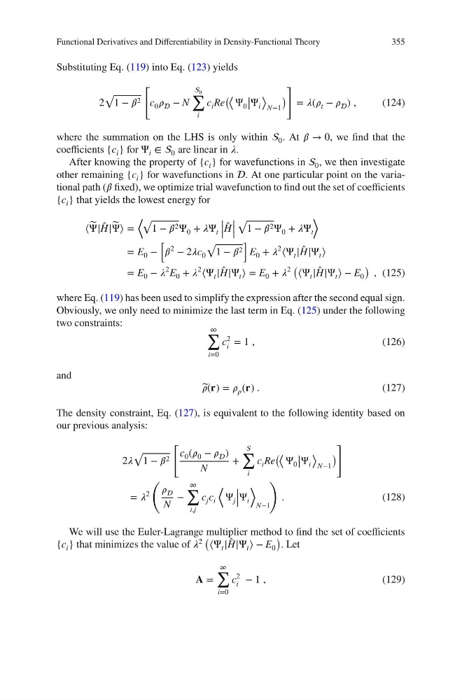
Substituting Eq. (119) into Eq. (123) yields
2
√
1 − í µí»½ 2
[
c 0 í µí¼ − N
0
∑
i
c i Re
(⟨ Ψ 0
|
| Ψ i
⟩
N−1
)
]
= í µí¼(í µí¼ t − í µí¼ ) ,
(124)
where the summation on the LHS is only within 0 . At í µí»½ → 0, we find that the
coefficients {c i } for Ψ i ∈ 0 are linear in í µí¼.
After knowing the property of {c i } for wavefunctions in 0 , we then investigate
other remaining {c i } for wavefunctions in . At one particular point on the variational path (í µí»½ fixed), we optimize trial wavefunction to find out the set of coefficients
{c i } that yields the lowest energy for
⟨ ̃
Ψ| ̂
H| ̃
Ψ⟩ =
⟨ √
1 − í µí»½ 2 Ψ 0 + í µí¼Ψ t
|
|
|
̂
H
|
|
|
√
1 − í µí»½ 2 Ψ 0 + í µí¼Ψ t
⟩
= E 0 −
[
í µí»½
2
− 2í µí¼c 0
√
1 − í µí»½ 2
]
E 0 + í µí¼
2
⟨Ψ t | ̂
H|Ψ t ⟩
= E 0 − í µí¼
2 E 0 + í µí¼
2
⟨Ψ t | ̂
H|Ψ t ⟩ = E 0 + í µí¼
2
( ⟨Ψ t | ̂
H|Ψ t ⟩ − E 0
) , (125)
where Eq. (119) has been used to simplify the expression after the second equal sign.
Obviously, we only need to minimize the last term in Eq. (125) under the following
two constraints:
∞
∑
i=0
c
2
i
= 1 ,
(126)
and
̃
í µí¼(í µí°«) = í µí¼ p (í µí°«) .
(127)
The density constraint, Eq. (127), is equivalent to the following identity based on
our previous analysis:
2í µí¼
√
1 − í µí»½ 2
[
c 0 (í µí¼ 0 − í µí¼ )
N
+
∑
i
c i Re
(⟨ Ψ 0
|
| Ψ i
⟩
N−1
)
]
= í µí¼
2
(
í µí¼
N
−
∞
∑
i,j
c j c i
⟨
Ψ j
|
|
|
Ψ i
⟩
N−1
)
.
(128)
We will use the Euler-Lagrange multiplier method to find the set of coefficients
{c i } that minimizes the value of í µí¼
2
( ⟨Ψ t | ̂
H|Ψ t ⟩ − E 0
)
. Let
í µí° =
∞
∑
i=0
c
2
i
− 1 ,
(129)
355
Substituting Eq. (119) into Eq. (123) yields
2
√
1 − í µí»½ 2
[
c 0 í µí¼ − N
0
∑
i
c i Re
(⟨ Ψ 0
|
| Ψ i
⟩
N−1
)
]
= í µí¼(í µí¼ t − í µí¼ ) ,
(124)
where the summation on the LHS is only within 0 . At í µí»½ → 0, we find that the
coefficients {c i } for Ψ i ∈ 0 are linear in í µí¼.
After knowing the property of {c i } for wavefunctions in 0 , we then investigate
other remaining {c i } for wavefunctions in . At one particular point on the variational path (í µí»½ fixed), we optimize trial wavefunction to find out the set of coefficients
{c i } that yields the lowest energy for
⟨ ̃
Ψ| ̂
H| ̃
Ψ⟩ =
⟨ √
1 − í µí»½ 2 Ψ 0 + í µí¼Ψ t
|
|
|
̂
H
|
|
|
√
1 − í µí»½ 2 Ψ 0 + í µí¼Ψ t
⟩
= E 0 −
[
í µí»½
2
− 2í µí¼c 0
√
1 − í µí»½ 2
]
E 0 + í µí¼
2
⟨Ψ t | ̂
H|Ψ t ⟩
= E 0 − í µí¼
2 E 0 + í µí¼
2
⟨Ψ t | ̂
H|Ψ t ⟩ = E 0 + í µí¼
2
( ⟨Ψ t | ̂
H|Ψ t ⟩ − E 0
) , (125)
where Eq. (119) has been used to simplify the expression after the second equal sign.
Obviously, we only need to minimize the last term in Eq. (125) under the following
two constraints:
∞
∑
i=0
c
2
i
= 1 ,
(126)
and
̃
í µí¼(í µí°«) = í µí¼ p (í µí°«) .
(127)
The density constraint, Eq. (127), is equivalent to the following identity based on
our previous analysis:
2í µí¼
√
1 − í µí»½ 2
[
c 0 (í µí¼ 0 − í µí¼ )
N
+
∑
i
c i Re
(⟨ Ψ 0
|
| Ψ i
⟩
N−1
)
]
= í µí¼
2
(
í µí¼
N
−
∞
∑
i,j
c j c i
⟨
Ψ j
|
|
|
Ψ i
⟩
N−1
)
.
(128)
We will use the Euler-Lagrange multiplier method to find the set of coefficients
{c i } that minimizes the value of í µí¼
2
( ⟨Ψ t | ̂
H|Ψ t ⟩ − E 0
)
. Let
í µí° =
∞
∑
i=0
c
2
i
− 1 ,
(129)