

354
P. Xiang and Y. A. Wang
following form:
̃
í µí¼(í µí°«) = N⟨ ̃
Ψ| ̃
Ψ⟩ N−1
= (1 − í µí»½
2
)N⟨Ψ 0 |Ψ 0 ⟩ N−1 + í µí¼
2 N⟨Ψ t |Ψ t ⟩ N−1 + 2í µí¼
√
1 − í µí»½ 2 NRe
( ⟨Ψ 0 |Ψ t ⟩ N−1
)
= (1 − í µí»½
2
)í µí¼ 0 (í µí°«) + í µí¼
2
í µí¼ t (í µí°«) + 2í µí¼
√
1 − í µí»½ 2 NRe
( ⟨Ψ 0 |Ψ t ⟩ N−1
) .
(116)
At any point, the trial density is identical to the path density to ensure that the density
variation is actually along the path we designed:
̃
í µí¼(í µí°«) = í µí¼ p (í µí°«) → í µí¼ 0 (í µí°«) .
(117)
Therefore, we have
⟨̃ í µí¼(í µí°«)⟩ =
⟨
í µí¼ p (í µí°«)
⟩ .
(118)
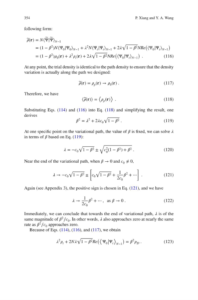
Substituting Eqs. (114) and (116) into Eq. (118) and simplifying the result, one
derives
í µí»½
2
= í µí¼
2
+ 2í µí¼c 0
√
1 − í µí»½ 2 .
(119)
At one specific point on the variational path, the value of í µí»½ is fixed, we can solve í µí¼
in terms of í µí»½ based on Eq. (119):
í µí¼ = −c 0
√
1 − í µí»½ 2 ±
√
c
2
0
(1 − í µí»½ 2 ) + í µí»½ 2 .
(120)
Near the end of the variational path, when í µí»½ → 0 and c 0 ≠ 0,
í µí¼ → −c 0
√
1 − í µí»½ 2 ±
[
c 0
√
1 − í µí»½ 2 +
1
2c 0
í µí»½
2
+ ⋯
]
.
(121)
Again (see Appendix 3), the positive sign is chosen in Eq. (121), and we have
í µí¼ →
1
2c 0
í µí»½
2
+ ⋯ , as í µí»½ → 0 .
(122)
Immediately, we can conclude that towards the end of variational path, í µí¼ is of the
same magnitude of í µí»½ 2 ∕c 0 . In other words, í µí¼ also approaches zero at nearly the same
rate as í µí»½ 2 ∕c 0 approaches zero.
Because of Eqs. (114), (116), and (117), we obtain
í µí¼
2
í µí¼ t + 2Ní µí¼
√
1 − í µí»½ 2 Re
(⟨ Ψ 0 |
| Ψ t
⟩
N−1
) = í µí»½
2
í µí¼ .
(123)
P. Xiang and Y. A. Wang
following form:
̃
í µí¼(í µí°«) = N⟨ ̃
Ψ| ̃
Ψ⟩ N−1
= (1 − í µí»½
2
)N⟨Ψ 0 |Ψ 0 ⟩ N−1 + í µí¼
2 N⟨Ψ t |Ψ t ⟩ N−1 + 2í µí¼
√
1 − í µí»½ 2 NRe
( ⟨Ψ 0 |Ψ t ⟩ N−1
)
= (1 − í µí»½
2
)í µí¼ 0 (í µí°«) + í µí¼
2
í µí¼ t (í µí°«) + 2í µí¼
√
1 − í µí»½ 2 NRe
( ⟨Ψ 0 |Ψ t ⟩ N−1
) .
(116)
At any point, the trial density is identical to the path density to ensure that the density
variation is actually along the path we designed:
̃
í µí¼(í µí°«) = í µí¼ p (í µí°«) → í µí¼ 0 (í µí°«) .
(117)
Therefore, we have
⟨̃ í µí¼(í µí°«)⟩ =
⟨
í µí¼ p (í µí°«)
⟩ .
(118)
Substituting Eqs. (114) and (116) into Eq. (118) and simplifying the result, one
derives
í µí»½
2
= í µí¼
2
+ 2í µí¼c 0
√
1 − í µí»½ 2 .
(119)
At one specific point on the variational path, the value of í µí»½ is fixed, we can solve í µí¼
in terms of í µí»½ based on Eq. (119):
í µí¼ = −c 0
√
1 − í µí»½ 2 ±
√
c
2
0
(1 − í µí»½ 2 ) + í µí»½ 2 .
(120)
Near the end of the variational path, when í µí»½ → 0 and c 0 ≠ 0,
í µí¼ → −c 0
√
1 − í µí»½ 2 ±
[
c 0
√
1 − í µí»½ 2 +
1
2c 0
í µí»½
2
+ ⋯
]
.
(121)
Again (see Appendix 3), the positive sign is chosen in Eq. (121), and we have
í µí¼ →
1
2c 0
í µí»½
2
+ ⋯ , as í µí»½ → 0 .
(122)
Immediately, we can conclude that towards the end of variational path, í µí¼ is of the
same magnitude of í µí»½ 2 ∕c 0 . In other words, í µí¼ also approaches zero at nearly the same
rate as í µí»½ 2 ∕c 0 approaches zero.
Because of Eqs. (114), (116), and (117), we obtain
í µí¼
2
í µí¼ t + 2Ní µí¼
√
1 − í µí»½ 2 Re
(⟨ Ψ 0 |
| Ψ t
⟩
N−1
) = í µí»½
2
í µí¼ .
(123)