

Theor Chem Acc (2015) 134:117
1 3
3.4 Bonds in molecules
One integral aspect of chemistry is that chemical bonds ,
formed from the interaction of electron density, hold the
atoms of a molecule together. Therefore, it is essential for
any AIM model to explicitly defi ne the bond.
We defi ne a bond as the region of space between a pair
of atoms where the joint probability of fi nding electron
density owned by each atom is nonzero. In the bonding
region, the weighting function of both nuclei ( W A and W B )
must be nonzero (and nonnegligible) since both the space
and electron density are shared. Thus, the bond density is
defi ned in Eq. 11 . Similarly, the radial bond density can be
defi ned as in Eq. 12 .
We denote the number of electrons in the bond A–B contributed from atom A as N A
A−B and calculate this value by
Eq. 13 . Therefore, the total number of bonding electrons in
A–B is the sum of the contributions from A and B as seen
in Eq. 14 . When performing the numerical integration for
Eq. 13 , we use the combined grid points of both atom A
and B .
(11)
ρ A−B (r) =
W A (r) W B (r) ρ(r)
(12)
ρ rad A−B (r) =
W A (r) W B (r) ρ rad (r)
The number of bonding electrons for several molecules is given in Table 4 , which show some very intuitive trends. First, for diatomics, the number of bonding electrons increases with increasing total charge as
seen by H
+
2 (0.34) < H 2 (0.71) < H
−
2 (0.79) . The addition of an electron to H 2 to form H
−
2 does not signifi -
cantly increase the number of bonding electrons, which
is the expected result from molecular orbital theory.
Another trend observed is the number of bonding electrons increases with bond order, such as the C–C bond in
H 3 C – CH 3 (1.65) < H 2 C=CH 2 (2.21) < HC≡CH (2.69).
Similarly, more electrons are observed in stronger bonds
than weaker bonds, such as: F 2 (2.12) < O 2 (2.58)
< CO (2.72) ≈ N 2 (2.81) . However, there are several
exceptions such as ClF (2.36), LiCl (2.56), and Cl 2 (2.68),
which do not follow these trends as discussed below.
Similar to AIM, we can also quantify the properties of
BIM. The shape, volume, and expectation values of BIM in
various molecules are calculated using either the RBCP or
DBCP as the origin as shown in Table 5 . Figure 7 shows
the shape and size of the bond density calculated at both the
RBCP and DBCP origin superimposed on a contour plot of
bond density for several diatomics. This fi gure reveals that
the RBCP origin better approximates bond density. Larger
versions for these diatomics, as well as three additional
examples, are shown in Figures S23–S29 of the supporting
information. Unfortunately, for a number of cases, the core
of the atom is included in the bond. This is an artifact of the
Becke weight, where the step function partitions the density
too early and causes the core to be included in the bond. As
observed in Fig. 7 , the Cl core contributes to the bond in
both ClF and LiCl, which results in the number of bonding
electrons in ClF (2.36) and LiCl (2.56) to be of the same
order as the double bond O 2 (2.58) as given in Table 4 .
One particularly interesting case is the hydrogenbridged B 2 H 6 molecule. A fi gure of the contours of radial
density for B 2 H 6 suggests that there is no B–B bond, as
shown in Figure S30 of the supporting information. This
is consistent with a QTAIM analysis which fi nds no bond
path between the boron atoms. Unfortunately, the machinery does not yet exist in MUNgauss to quantitatively calculate the number of bonding electrons for 3-centered
bonds.
3.5 Applications
Is molecular radial density chemically signifi cant? One
application is predicting the orientation of molecular
(13)
N
A
A−B =
W A (r) ρ A−B (r)dr
(14)
N A−B = N
A
A−B + N
B
A−B
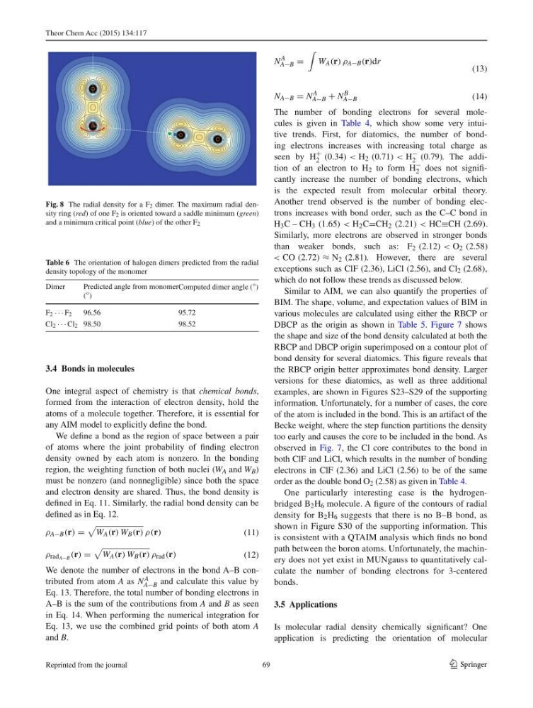
Fig. 8 The radial density for a F 2 dimer. The maximum radial density ring ( red ) of one F 2 is oriented toward a saddle minimum ( green )
and a minimum critical point ( blue ) of the other F 2
Table 6 The orientation of halogen dimers predicted from the radial
density topology of the monomer
Dimer
Predicted angle from monomer
(
◦ )
Computed dimer angle (
◦ )
F 2 · · · F 2
96.56
95.72
Cl 2 · · · Cl 2 98.50
98.52
69
Reprinted from the journal
1 3
3.4 Bonds in molecules
One integral aspect of chemistry is that chemical bonds ,
formed from the interaction of electron density, hold the
atoms of a molecule together. Therefore, it is essential for
any AIM model to explicitly defi ne the bond.
We defi ne a bond as the region of space between a pair
of atoms where the joint probability of fi nding electron
density owned by each atom is nonzero. In the bonding
region, the weighting function of both nuclei ( W A and W B )
must be nonzero (and nonnegligible) since both the space
and electron density are shared. Thus, the bond density is
defi ned in Eq. 11 . Similarly, the radial bond density can be
defi ned as in Eq. 12 .
We denote the number of electrons in the bond A–B contributed from atom A as N A
A−B and calculate this value by
Eq. 13 . Therefore, the total number of bonding electrons in
A–B is the sum of the contributions from A and B as seen
in Eq. 14 . When performing the numerical integration for
Eq. 13 , we use the combined grid points of both atom A
and B .
(11)
ρ A−B (r) =
W A (r) W B (r) ρ(r)
(12)
ρ rad A−B (r) =
W A (r) W B (r) ρ rad (r)
The number of bonding electrons for several molecules is given in Table 4 , which show some very intuitive trends. First, for diatomics, the number of bonding electrons increases with increasing total charge as
seen by H
+
2 (0.34) < H 2 (0.71) < H
−
2 (0.79) . The addition of an electron to H 2 to form H
−
2 does not signifi -
cantly increase the number of bonding electrons, which
is the expected result from molecular orbital theory.
Another trend observed is the number of bonding electrons increases with bond order, such as the C–C bond in
H 3 C – CH 3 (1.65) < H 2 C=CH 2 (2.21) < HC≡CH (2.69).
Similarly, more electrons are observed in stronger bonds
than weaker bonds, such as: F 2 (2.12) < O 2 (2.58)
< CO (2.72) ≈ N 2 (2.81) . However, there are several
exceptions such as ClF (2.36), LiCl (2.56), and Cl 2 (2.68),
which do not follow these trends as discussed below.
Similar to AIM, we can also quantify the properties of
BIM. The shape, volume, and expectation values of BIM in
various molecules are calculated using either the RBCP or
DBCP as the origin as shown in Table 5 . Figure 7 shows
the shape and size of the bond density calculated at both the
RBCP and DBCP origin superimposed on a contour plot of
bond density for several diatomics. This fi gure reveals that
the RBCP origin better approximates bond density. Larger
versions for these diatomics, as well as three additional
examples, are shown in Figures S23–S29 of the supporting
information. Unfortunately, for a number of cases, the core
of the atom is included in the bond. This is an artifact of the
Becke weight, where the step function partitions the density
too early and causes the core to be included in the bond. As
observed in Fig. 7 , the Cl core contributes to the bond in
both ClF and LiCl, which results in the number of bonding
electrons in ClF (2.36) and LiCl (2.56) to be of the same
order as the double bond O 2 (2.58) as given in Table 4 .
One particularly interesting case is the hydrogenbridged B 2 H 6 molecule. A fi gure of the contours of radial
density for B 2 H 6 suggests that there is no B–B bond, as
shown in Figure S30 of the supporting information. This
is consistent with a QTAIM analysis which fi nds no bond
path between the boron atoms. Unfortunately, the machinery does not yet exist in MUNgauss to quantitatively calculate the number of bonding electrons for 3-centered
bonds.
3.5 Applications
Is molecular radial density chemically signifi cant? One
application is predicting the orientation of molecular
(13)
N
A
A−B =
W A (r) ρ A−B (r)dr
(14)
N A−B = N
A
A−B + N
B
A−B
Fig. 8 The radial density for a F 2 dimer. The maximum radial density ring ( red ) of one F 2 is oriented toward a saddle minimum ( green )
and a minimum critical point ( blue ) of the other F 2
Table 6 The orientation of halogen dimers predicted from the radial
density topology of the monomer
Dimer
Predicted angle from monomer
(
◦ )
Computed dimer angle (
◦ )
F 2 · · · F 2
96.56
95.72
Cl 2 · · · Cl 2 98.50
98.52
69
Reprinted from the journal