

Theor Chem Acc (2015) 134:74
1 3
momentum quantum number of the functions is in average
signifi cantly lower: There is no d function in the basis sets,
and the number of p functions is also considerably lower.
3 Bond-centered general ellipsoidal Gaussian
functions
In this section, we study an extension of the BF approach.
Only BF basis sets including s -type functions will be considered, but instead of the conventional, spherical Gaussians BC ellipsoidal Gaussians of general form will be
employed. Since such functions, to the best of our knowledge, have not yet been considered in quantum chemistry,
fi rst, we briefl y discuss how the integrals over ellipsoidal
Gaussians can be evaluated and what modifi cations in a
quantum chemistry program are required to process such
functions. Second, we will examine to what extent the
additional fl exibility of ellipsoidal functions with respect to
conventional Gaussians improves the calculated energies.
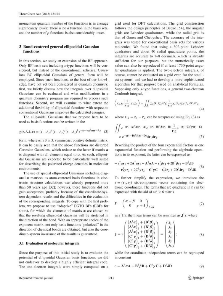
The ellipsoidal Gaussians that we propose here to be
used as basis functions can be written in the
form, where α is 3 × 3, symmetric, positive defi nite matrix.
It can be easily seen that the above functions are distorted
Cartesian Gaussians, which reduce to the latter if matrix α
is diagonal with all elements equal to α . As such, ellipsoidal Gaussians are expected to be particularly well suited
for describing the polarized charge densities in molecular
environments.
The use of special ellipsoidal Gaussians including diagonal α matrices as atom-centered basis functions in electronic structure calculations was already proposed more
than 50 years ago [ 32 ]; however, these functions did not
gain acceptance, probably because of the coordinate-system-dependent results and the diffi culties in the evaluation
of the corresponding integrals. To cope with the fi rst problem, we propose to use “adaptive” EGTO BFs (EBFs for
short), for which the elements of matrix α are chosen so
that the resulting ellipsoidal Gaussian will be stretched in
the direction of the bond. With an appropriate choice of the
exponent matrix, not only basis functions “polarized” in the
direction of chemical bonds are obtained, but also the coordinate-system invariance of the results is guaranteed.
3.1 Evaluation of molecular integrals
Since the purpose of this initial study is to evaluate the
potential of ellipsoidal Gaussian basis functions, we did
not endeavor to develop a highly effi cient integral code.
The one-electron integrals were simply computed on a
(3)
χ (r, A, l, α) = (x − A x ) i
y − A y
j (z − A z ) k e −(r−A) † α(r−A)
grid used for DFT calculations. The grid construction
follows the design principles of Becke [ 54 ], the angular
grids are Lebedev quadratures, while the radial grid is
that of Gauss and Chebyshev. The accuracy of the integrals was tested for conventional basis sets for various
molecules. We found that using a 302-point Lebedev
quadrature and about 40 radial quadrature points, the
integrals are accurate to 7–8 decimals, which is already
suffi cient for our purposes, but the numerically exact
value can also be reproduced if at least 1730-point angular quadrature is applied. The two-electron integrals, of
course, cannot be evaluated on a grid even for the smallest systems, and we had to develop a more sophisticated
algorithm for that purpose based on analytical formulas.
Supposing only s -type functions, a general two-electron
Coulomb integral,
where r 12 = r 1 − r 2 , can be reexpressed using Eq. ( 3 ) as
Rewriting the product of the four exponential factors as one
exponential function and performing the algebraic operations in its exponent, the latter can be expressed as
To further simplify the expression, we introduce the
r = (r 1 , r 2 ) six-component vector containing the electronic coordinates. The terms that are quadratic in r can be
expressed with the aid of a 6 × 6 matrix
as r † r; the linear terms can be rewritten as J † r, where
while the coordinate-independent terms can be regrouped
in constant
(4)
χ μ χ ν
1
r 12
χ χ σ
=
χ μ (r 1 )χ ν (r 1 )
1
r 12
χ (r 2 )χ σ (r 2 )dr 1 dr 2 ,
(5)
e
−(r 1 −A) † α(r 1 −A) e
−(r 1 −B) † β(r 1 −B) 1
r 12
e
−(r 2 −C) † γ (r 2 −C)
× e
−(r 2 −D) † δ(r 2 −D) dr 1 dr 2 .
(6)
− r
†
1 αr 1 + 2A † αr 1 − A † αA − r
†
1 βr 1 + 2B † βr 1 − B † βB
− r
†
2 γ r 2 + 2C † γ r 2 − C † γ C − r
†
2 δr 2 + 2D † δr 2 − D † δD.
(7)
=
α + β 0
0 γ + δ
6×6
(8)
J = 2
⎛
⎜
⎜
⎜
⎜
⎜
⎜
⎝
A † α
1
+
B † β
1
A † α
2
+
B † β
2
A † α
3
+
B † β
3
C † γ
1
+
D † δ
1
C † γ
2
+
D † δ
2
C † γ
3
+
D † δ
3
⎞
⎟
⎟
⎟
⎟
⎟
⎟
⎠
=
⎛
⎜
⎜
⎜
⎜
⎜
⎜
⎝
J 1
J 2
J 3
J 4
J 5
J 6
⎞
⎟
⎟
⎟
⎟
⎟
⎟
⎠
;
(9)
c = A
†
αA + B
†
βB + C
†
γ C + D
†
δD.
213
Reprinted from the journal
1 3
momentum quantum number of the functions is in average
signifi cantly lower: There is no d function in the basis sets,
and the number of p functions is also considerably lower.
3 Bond-centered general ellipsoidal Gaussian
functions
In this section, we study an extension of the BF approach.
Only BF basis sets including s -type functions will be considered, but instead of the conventional, spherical Gaussians BC ellipsoidal Gaussians of general form will be
employed. Since such functions, to the best of our knowledge, have not yet been considered in quantum chemistry,
fi rst, we briefl y discuss how the integrals over ellipsoidal
Gaussians can be evaluated and what modifi cations in a
quantum chemistry program are required to process such
functions. Second, we will examine to what extent the
additional fl exibility of ellipsoidal functions with respect to
conventional Gaussians improves the calculated energies.
The ellipsoidal Gaussians that we propose here to be
used as basis functions can be written in the
form, where α is 3 × 3, symmetric, positive defi nite matrix.
It can be easily seen that the above functions are distorted
Cartesian Gaussians, which reduce to the latter if matrix α
is diagonal with all elements equal to α . As such, ellipsoidal Gaussians are expected to be particularly well suited
for describing the polarized charge densities in molecular
environments.
The use of special ellipsoidal Gaussians including diagonal α matrices as atom-centered basis functions in electronic structure calculations was already proposed more
than 50 years ago [ 32 ]; however, these functions did not
gain acceptance, probably because of the coordinate-system-dependent results and the diffi culties in the evaluation
of the corresponding integrals. To cope with the fi rst problem, we propose to use “adaptive” EGTO BFs (EBFs for
short), for which the elements of matrix α are chosen so
that the resulting ellipsoidal Gaussian will be stretched in
the direction of the bond. With an appropriate choice of the
exponent matrix, not only basis functions “polarized” in the
direction of chemical bonds are obtained, but also the coordinate-system invariance of the results is guaranteed.
3.1 Evaluation of molecular integrals
Since the purpose of this initial study is to evaluate the
potential of ellipsoidal Gaussian basis functions, we did
not endeavor to develop a highly effi cient integral code.
The one-electron integrals were simply computed on a
(3)
χ (r, A, l, α) = (x − A x ) i
y − A y
j (z − A z ) k e −(r−A) † α(r−A)
grid used for DFT calculations. The grid construction
follows the design principles of Becke [ 54 ], the angular
grids are Lebedev quadratures, while the radial grid is
that of Gauss and Chebyshev. The accuracy of the integrals was tested for conventional basis sets for various
molecules. We found that using a 302-point Lebedev
quadrature and about 40 radial quadrature points, the
integrals are accurate to 7–8 decimals, which is already
suffi cient for our purposes, but the numerically exact
value can also be reproduced if at least 1730-point angular quadrature is applied. The two-electron integrals, of
course, cannot be evaluated on a grid even for the smallest systems, and we had to develop a more sophisticated
algorithm for that purpose based on analytical formulas.
Supposing only s -type functions, a general two-electron
Coulomb integral,
where r 12 = r 1 − r 2 , can be reexpressed using Eq. ( 3 ) as
Rewriting the product of the four exponential factors as one
exponential function and performing the algebraic operations in its exponent, the latter can be expressed as
To further simplify the expression, we introduce the
r = (r 1 , r 2 ) six-component vector containing the electronic coordinates. The terms that are quadratic in r can be
expressed with the aid of a 6 × 6 matrix
as r † r; the linear terms can be rewritten as J † r, where
while the coordinate-independent terms can be regrouped
in constant
(4)
χ μ χ ν
1
r 12
χ χ σ
=
χ μ (r 1 )χ ν (r 1 )
1
r 12
χ (r 2 )χ σ (r 2 )dr 1 dr 2 ,
(5)
e
−(r 1 −A) † α(r 1 −A) e
−(r 1 −B) † β(r 1 −B) 1
r 12
e
−(r 2 −C) † γ (r 2 −C)
× e
−(r 2 −D) † δ(r 2 −D) dr 1 dr 2 .
(6)
− r
†
1 αr 1 + 2A † αr 1 − A † αA − r
†
1 βr 1 + 2B † βr 1 − B † βB
− r
†
2 γ r 2 + 2C † γ r 2 − C † γ C − r
†
2 δr 2 + 2D † δr 2 − D † δD.
(7)
=
α + β 0
0 γ + δ
6×6
(8)
J = 2
⎛
⎜
⎜
⎜
⎜
⎜
⎜
⎝
A † α
1
+
B † β
1
A † α
2
+
B † β
2
A † α
3
+
B † β
3
C † γ
1
+
D † δ
1
C † γ
2
+
D † δ
2
C † γ
3
+
D † δ
3
⎞
⎟
⎟
⎟
⎟
⎟
⎟
⎠
=
⎛
⎜
⎜
⎜
⎜
⎜
⎜
⎝
J 1
J 2
J 3
J 4
J 5
J 6
⎞
⎟
⎟
⎟
⎟
⎟
⎟
⎠
;
(9)
c = A
†
αA + B
†
βB + C
†
γ C + D
†
δD.
213
Reprinted from the journal