

Theor Chem Acc (2015) 134:148
1 3
convergence, we could transform the amplitudes back to
the original POO basis according to:
However, this back-transformation is not necessary
since the correlation energy can be obtained directly in the
pseudo-canonical basis, as:
Appendix 4: Riccati equations in the local
excitation approximation
The local excitation approximation imposes that in the
matrices R , , A and B , the excitations remain on the same
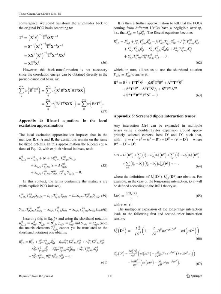
localized orbitals. In this approximation the Riccati equations of Eq. 12 , with explicit virtual indexes, read:
In this context, the terms containing the matrix are
(with explicit POO indexes):
Inserting this in Eq. 58 and using the shorthand notation
R
ij
i α j β
≡ R
ij
αβ , B
ij
i α j β
≡ B
ij
αβ , f i α j β ≡ f
ij
αβ and S i α j β ≡ S
ij
αβ , (note
the matrix elements T
ij
i γ p δ
cannot yet be translated to the
shorthand notation) one obtains:
(56)
T
ij
=
X
† S
−1
T
ij (SX)
−1
= S
−1
X
†
−1
T
ij X
−1 S
−1
= XX
†
X
†
−1
T
ij X
−1 XX
†
= XT
ij X
† .
(57)
occ
ij
tr
B
ij T
ij
=
occ
ij
tr
X
† B
ij XX
† ST
ij SX
=
occ
ij
tr
B
ij T
ij SXX
†
=
occ
ij
tr
B
ij T
ij
.
(58)
R
ij
i α j β
= B
ij
i α j β
+ (( + A)
im
i α m γ
T
mj
m γ p δ
S p δ j β
+ S i α p γ T
im
p γ m δ
(( + A)
mj
m δ j β
+ S i α p γ T
im
p γ m δ
B
mn
m δ n τ
T
nj
n τ q ζ
S q ζ j β = 0.
(59)
im
i α m γ
T
mj
m γ p δ
S p δ j β = f i α i γ T
ij
i γ p δ
S p δ j β − f im S i α m γ T
mj
m γ p δ
S p δ j β
(60)
S i α p γ T
im
p γ m δ
mj
m δ j β
= S i α p γ T
ij
p γ j δ
f j δ j β − S i α p γ T
im
p γ m δ
S m δ j β f mj .
(61)
R
ij
αβ = B
ij
αβ + f ii
αγ T
ij
i γ p δ
S
pj
δβ − f im S im
αγ T
mj
m γ p δ S
pj
δβ + A im
αγ T
mj
m γ p δ S
pj
δβ
+ S
ip
αγ T
ij
p γ j δ
f
jj
δβ − S
ip
αγ T im
p γ m δ S
mj
δβ f mj + S
ip
αγ T im
p γ m δ A
mj
δβ
+ S
ip
αγ T im
p γ m δ B mn
δτ T
nj
n τ q ζ S
qj
ζβ = 0.
It is then a further approximation to tell that the POOs
coming from different LMOs have a negligible overlap,
i.e., that S
ij
αβ = δ ij S ii
αβ . The Riccati equations become:
which, in turn, allows us to use the shorthand notation
T i α j β ≡ T
ij
αβ to arrive at:
Appendix 5: Screened dipole interaction tensor
Any interaction L(r) can be expanded in multipole
series using a double Taylor expansion around appropriately selected centers, here D i and D j , such that,
with r = r i − r j = (r i − D i ) + D ij − (r j − D j ) where
D ij = D i − D j :
where the defi nitions of L
ij
α (D ij ) , L
ij
αβ (D ij ) are obvious. For
example, in the case of the long-range interaction, L(r) will
be defi ned according to the RSH theory as:
with r = |r|.
The multipolar expansion of the long-range interaction
leads to the following fi rst and second-order interaction
tensors:
(62)
R
ij
αβ = B
ij
αβ + f
ii
αγ T
ij
i γ j δ
S
jj
δβ − f ii S
ii
αγ T
ij
i γ j δ
S
jj
δβ + A
im
αγ T
mj
m γ j δ
S
jj
δβ
+ S
ii
αγ T
ij
i γ j δ
f
jj
δβ − S
ii
αγ T
ij
i γ j δ
S
jj
δβ f jj + S
ii
αγ T
im
i γ m δ
A
mj
δβ
+ S
ii
αγ T
im
i γ m δ
B
mn
δτ T
nj
n τ j ζ
S
jj
ζβ = 0,
(63)
R
ij
= B
ij
+ f
ii T
ij S
jj
− f ii S
ii T
ij S
jj
+ A
im T
mj S
jj
+ S
ii T
ij f
jj
− S
ii T
ij S
jj f jj + S
ii T
im A
mj
+ S
ii T
im B
mn T
nj S
jj
= 0,
(64)
L(r) = L ij
D ij
+
α
ˆ
r i
α − D i
α
L
ij
α
D ij
+
α
ˆ
r
j
α − D
j
α
L
ij
α
D ij
+
αβ
ˆ
r i
α − D i
α
ˆ
r
j
β − D
j
β
L
ij
αβ
D ij
+ · · · ,
(65)
L(r) =
erf(μr)
r
,
(66)
L
ij
α
D
ij
= −
D
ij
α
D ij 3
1 −
2
√
π
D
ij
μe
−μ 2 D ij 2 − erf
μD
ij
(67)
L
ij
αβ
D
ij
=
3D
ij
α D
ij
β
D ij 5
erf
μD
ij
−
2
3
√
π
D
ij μe
−μ 2 D ij 2
3 + 2D
ij 2 μ
2
−
δ αβ D ij 2
D ij 5
erf
μD
ij
−
2
√
π
D
ij μe
−μ 2 D ij 2
.
111
Reprinted from the journal
1 3
convergence, we could transform the amplitudes back to
the original POO basis according to:
However, this back-transformation is not necessary
since the correlation energy can be obtained directly in the
pseudo-canonical basis, as:
Appendix 4: Riccati equations in the local
excitation approximation
The local excitation approximation imposes that in the
matrices R , , A and B , the excitations remain on the same
localized orbitals. In this approximation the Riccati equations of Eq. 12 , with explicit virtual indexes, read:
In this context, the terms containing the matrix are
(with explicit POO indexes):
Inserting this in Eq. 58 and using the shorthand notation
R
ij
i α j β
≡ R
ij
αβ , B
ij
i α j β
≡ B
ij
αβ , f i α j β ≡ f
ij
αβ and S i α j β ≡ S
ij
αβ , (note
the matrix elements T
ij
i γ p δ
cannot yet be translated to the
shorthand notation) one obtains:
(56)
T
ij
=
X
† S
−1
T
ij (SX)
−1
= S
−1
X
†
−1
T
ij X
−1 S
−1
= XX
†
X
†
−1
T
ij X
−1 XX
†
= XT
ij X
† .
(57)
occ
ij
tr
B
ij T
ij
=
occ
ij
tr
X
† B
ij XX
† ST
ij SX
=
occ
ij
tr
B
ij T
ij SXX
†
=
occ
ij
tr
B
ij T
ij
.
(58)
R
ij
i α j β
= B
ij
i α j β
+ (( + A)
im
i α m γ
T
mj
m γ p δ
S p δ j β
+ S i α p γ T
im
p γ m δ
(( + A)
mj
m δ j β
+ S i α p γ T
im
p γ m δ
B
mn
m δ n τ
T
nj
n τ q ζ
S q ζ j β = 0.
(59)
im
i α m γ
T
mj
m γ p δ
S p δ j β = f i α i γ T
ij
i γ p δ
S p δ j β − f im S i α m γ T
mj
m γ p δ
S p δ j β
(60)
S i α p γ T
im
p γ m δ
mj
m δ j β
= S i α p γ T
ij
p γ j δ
f j δ j β − S i α p γ T
im
p γ m δ
S m δ j β f mj .
(61)
R
ij
αβ = B
ij
αβ + f ii
αγ T
ij
i γ p δ
S
pj
δβ − f im S im
αγ T
mj
m γ p δ S
pj
δβ + A im
αγ T
mj
m γ p δ S
pj
δβ
+ S
ip
αγ T
ij
p γ j δ
f
jj
δβ − S
ip
αγ T im
p γ m δ S
mj
δβ f mj + S
ip
αγ T im
p γ m δ A
mj
δβ
+ S
ip
αγ T im
p γ m δ B mn
δτ T
nj
n τ q ζ S
qj
ζβ = 0.
It is then a further approximation to tell that the POOs
coming from different LMOs have a negligible overlap,
i.e., that S
ij
αβ = δ ij S ii
αβ . The Riccati equations become:
which, in turn, allows us to use the shorthand notation
T i α j β ≡ T
ij
αβ to arrive at:
Appendix 5: Screened dipole interaction tensor
Any interaction L(r) can be expanded in multipole
series using a double Taylor expansion around appropriately selected centers, here D i and D j , such that,
with r = r i − r j = (r i − D i ) + D ij − (r j − D j ) where
D ij = D i − D j :
where the defi nitions of L
ij
α (D ij ) , L
ij
αβ (D ij ) are obvious. For
example, in the case of the long-range interaction, L(r) will
be defi ned according to the RSH theory as:
with r = |r|.
The multipolar expansion of the long-range interaction
leads to the following fi rst and second-order interaction
tensors:
(62)
R
ij
αβ = B
ij
αβ + f
ii
αγ T
ij
i γ j δ
S
jj
δβ − f ii S
ii
αγ T
ij
i γ j δ
S
jj
δβ + A
im
αγ T
mj
m γ j δ
S
jj
δβ
+ S
ii
αγ T
ij
i γ j δ
f
jj
δβ − S
ii
αγ T
ij
i γ j δ
S
jj
δβ f jj + S
ii
αγ T
im
i γ m δ
A
mj
δβ
+ S
ii
αγ T
im
i γ m δ
B
mn
δτ T
nj
n τ j ζ
S
jj
ζβ = 0,
(63)
R
ij
= B
ij
+ f
ii T
ij S
jj
− f ii S
ii T
ij S
jj
+ A
im T
mj S
jj
+ S
ii T
ij f
jj
− S
ii T
ij S
jj f jj + S
ii T
im A
mj
+ S
ii T
im B
mn T
nj S
jj
= 0,
(64)
L(r) = L ij
D ij
+
α
ˆ
r i
α − D i
α
L
ij
α
D ij
+
α
ˆ
r
j
α − D
j
α
L
ij
α
D ij
+
αβ
ˆ
r i
α − D i
α
ˆ
r
j
β − D
j
β
L
ij
αβ
D ij
+ · · · ,
(65)
L(r) =
erf(μr)
r
,
(66)
L
ij
α
D
ij
= −
D
ij
α
D ij 3
1 −
2
√
π
D
ij
μe
−μ 2 D ij 2 − erf
μD
ij
(67)
L
ij
αβ
D
ij
=
3D
ij
α D
ij
β
D ij 5
erf
μD
ij
−
2
3
√
π
D
ij μe
−μ 2 D ij 2
3 + 2D
ij 2 μ
2
−
δ αβ D ij 2
D ij 5
erf
μD
ij
−
2
√
π
D
ij μe
−μ 2 D ij 2
.
111
Reprinted from the journal