

Theor Chem Acc (2015) 134:148
1 3
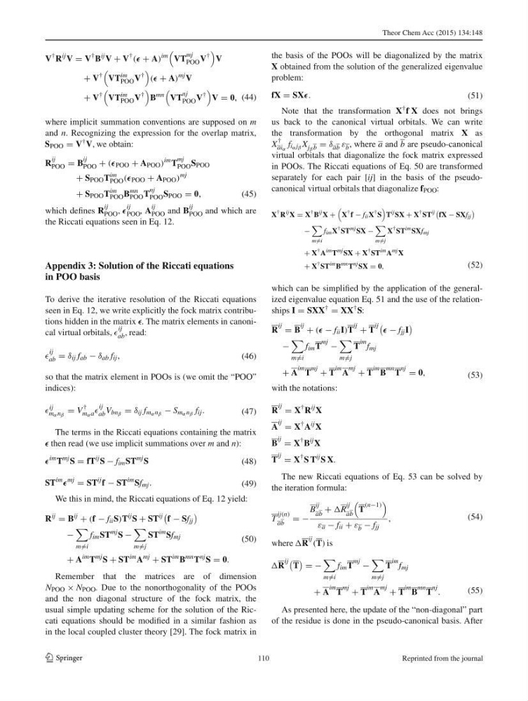
where implicit summation conventions are supposed on m
and n . Recognizing the expression for the overlap matrix,
S POO = V † V, we obtain:
which defi nes R
ij
POO ,
ij
POO , A
ij
POO and B
ij
POO and which are
the Riccati equations seen in Eq. 12 .
Appendix 3: Solution of the Riccati equations
in POO basis
To derive the iterative resolution of the Riccati equations
seen in Eq. 12 , we write explicitly the fock matrix contributions hidden in the matrix . The matrix elements in canonical virtual orbitals,
ij
ab , read:
so that the matrix element in POOs is (we omit the “POO”
indices):
The terms in the Riccati equations containing the matrix
then read (we use implicit summations over m and n ):
We this in mind, the Riccati equations of Eq. 12 yield:
Remember that the matrices are of dimension
N POO × N POO . Due to the nonorthogonality of the POOs
and the non diagonal structure of the fock matrix, the
usual simple updating scheme for the solution of the Riccati equations should be modifi ed in a similar fashion as
in the local coupled cluster theory [ 29 ]. The fock matrix in
(44)
V
† R
ij V = V
† B
ij V + V
†
( + A)
im
VT
mj
POO V
†
V
+ V
†
VT
im
POO V
†
( + A)
mj V
+ V
†
VT
im
POO V
†
B
mn
VT
nj
POO V
†
V = 0,
(45)
R
ij
POO = B
ij
POO + ( POO + A POO )
im T
mj
POO S POO
+ S POO T
im
POO ( POO + A POO )
mj
+ S POO T
im
POO B
mn
POO T
nj
POO S POO = 0,
(46)
ij
ab = δ ij f ab − δ ab f ij ,
(47)
ij
m α n β
= V
†
m α a
ij
ab V bn β = δ ij f m α n β − S m α n β f ij .
(48)
im T
mj S = fT
ij S − f im ST
mj S
(49)
ST
im
mj
= ST
ij f − ST
im Sf mj .
(50)
R
ij
= B
ij
+ (f − f ii S)T
ij S + ST
ij
f − Sf jj
−
m =i
f im ST
mj S −
m =j
ST
im Sf mj
+ A
im T
mj S + ST
im A
mj
+ ST
im B
mn T
nj S = 0.
the basis of the POOs will be diagonalized by the matrix
X obtained from the solution of the generalized eigenvalue
problem:
Note that the transformation X † f X does not brings
us back to the canonical virtual orbitals. We can write
the transformation by the orthogonal matrix X as
X
†
ai α
f i α j β X j β b = δ ab ε b , where a and b are pseudo-canonical
virtual orbitals that diagonalize the fock matrix expressed
in POOs. The Riccati equations of Eq. 50 are transformed
separately for each pair [ ij ] in the basis of the pseudocanonical virtual orbitals that diagonalize f POO :
which can be simplifi ed by the application of the generalized eigenvalue equation Eq. 51 and the use of the relationships I = SXX † = XX † S :
with the notations:
The new Riccati equations of Eq. 53 can be solved by
the iteration formula:
where R
ij (T) is
As presented here, the update of the “non-diagonal” part
of the residue is done in the pseudo-canonical basis. After
(51)
fX = SX.
(52)
X
† R
ij X = X
† B
ij X +
X
† f − f ii X
† S
T
ij SX + X
† ST
ij
fX − SXf jj
−
m =i
f im X
† ST
mj SX −
m =j
X
† ST
im SXf mj
+ X
† A
im T
mj SX + X
† ST
im A
mj X
+ X
† ST
im B
mn T
nj SX = 0,
(53)
R
ij = B
ij + ( − f ii I)T
ij + T
ij − f jj I
−
m =i
f im T
mj −
m =j
T
im f mj
+ A
im T
mj + T
im A
mj + T
im B
mn T
nj = 0,
R
ij = X
† R
ij X
A
ij = X
† A
ij X
B
ij = X
† B
ij X
T
ij = X
† S T
ij S X.
(54)
T
ij(n)
ab
= −
B
ij
ab
+ R
ij
ab
T
(n−1)
ε a − f ii + ε b − f jj
,
(55)
R
ij
T
= −
m =i
f im T
mj −
m =j
T
im f mj
+ A
im T
mj + T
im A
mj + T
im B
mn T
nj .
110
Reprinted from the journal
1 3
where implicit summation conventions are supposed on m
and n . Recognizing the expression for the overlap matrix,
S POO = V † V, we obtain:
which defi nes R
ij
POO ,
ij
POO , A
ij
POO and B
ij
POO and which are
the Riccati equations seen in Eq. 12 .
Appendix 3: Solution of the Riccati equations
in POO basis
To derive the iterative resolution of the Riccati equations
seen in Eq. 12 , we write explicitly the fock matrix contributions hidden in the matrix . The matrix elements in canonical virtual orbitals,
ij
ab , read:
so that the matrix element in POOs is (we omit the “POO”
indices):
The terms in the Riccati equations containing the matrix
then read (we use implicit summations over m and n ):
We this in mind, the Riccati equations of Eq. 12 yield:
Remember that the matrices are of dimension
N POO × N POO . Due to the nonorthogonality of the POOs
and the non diagonal structure of the fock matrix, the
usual simple updating scheme for the solution of the Riccati equations should be modifi ed in a similar fashion as
in the local coupled cluster theory [ 29 ]. The fock matrix in
(44)
V
† R
ij V = V
† B
ij V + V
†
( + A)
im
VT
mj
POO V
†
V
+ V
†
VT
im
POO V
†
( + A)
mj V
+ V
†
VT
im
POO V
†
B
mn
VT
nj
POO V
†
V = 0,
(45)
R
ij
POO = B
ij
POO + ( POO + A POO )
im T
mj
POO S POO
+ S POO T
im
POO ( POO + A POO )
mj
+ S POO T
im
POO B
mn
POO T
nj
POO S POO = 0,
(46)
ij
ab = δ ij f ab − δ ab f ij ,
(47)
ij
m α n β
= V
†
m α a
ij
ab V bn β = δ ij f m α n β − S m α n β f ij .
(48)
im T
mj S = fT
ij S − f im ST
mj S
(49)
ST
im
mj
= ST
ij f − ST
im Sf mj .
(50)
R
ij
= B
ij
+ (f − f ii S)T
ij S + ST
ij
f − Sf jj
−
m =i
f im ST
mj S −
m =j
ST
im Sf mj
+ A
im T
mj S + ST
im A
mj
+ ST
im B
mn T
nj S = 0.
the basis of the POOs will be diagonalized by the matrix
X obtained from the solution of the generalized eigenvalue
problem:
Note that the transformation X † f X does not brings
us back to the canonical virtual orbitals. We can write
the transformation by the orthogonal matrix X as
X
†
ai α
f i α j β X j β b = δ ab ε b , where a and b are pseudo-canonical
virtual orbitals that diagonalize the fock matrix expressed
in POOs. The Riccati equations of Eq. 50 are transformed
separately for each pair [ ij ] in the basis of the pseudocanonical virtual orbitals that diagonalize f POO :
which can be simplifi ed by the application of the generalized eigenvalue equation Eq. 51 and the use of the relationships I = SXX † = XX † S :
with the notations:
The new Riccati equations of Eq. 53 can be solved by
the iteration formula:
where R
ij (T) is
As presented here, the update of the “non-diagonal” part
of the residue is done in the pseudo-canonical basis. After
(51)
fX = SX.
(52)
X
† R
ij X = X
† B
ij X +
X
† f − f ii X
† S
T
ij SX + X
† ST
ij
fX − SXf jj
−
m =i
f im X
† ST
mj SX −
m =j
X
† ST
im SXf mj
+ X
† A
im T
mj SX + X
† ST
im A
mj X
+ X
† ST
im B
mn T
nj SX = 0,
(53)
R
ij = B
ij + ( − f ii I)T
ij + T
ij − f jj I
−
m =i
f im T
mj −
m =j
T
im f mj
+ A
im T
mj + T
im A
mj + T
im B
mn T
nj = 0,
R
ij = X
† R
ij X
A
ij = X
† A
ij X
B
ij = X
† B
ij X
T
ij = X
† S T
ij S X.
(54)
T
ij(n)
ab
= −
B
ij
ab
+ R
ij
ab
T
(n−1)
ε a − f ii + ε b − f jj
,
(55)
R
ij
T
= −
m =i
f im T
mj −
m =j
T
im f mj
+ A
im T
mj + T
im A
mj + T
im B
mn T
nj .
110
Reprinted from the journal