

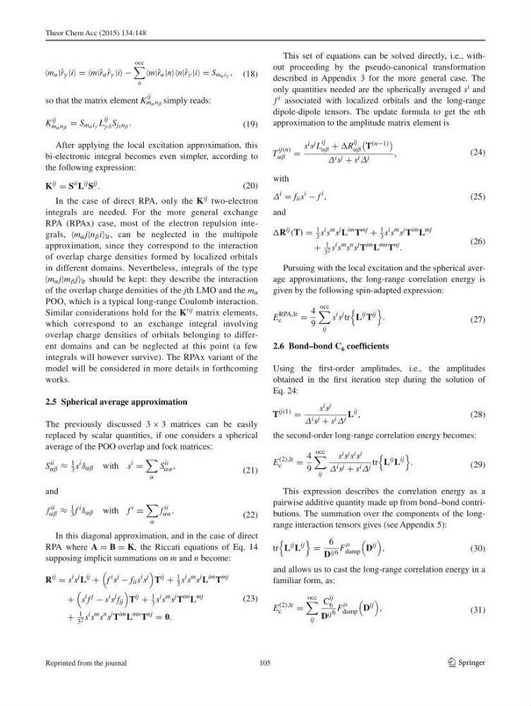
Theor Chem Acc (2015) 134:148
1 3
so that the matrix element K
ij
m α n β simply reads:
After applying the local excitation approximation, this
bi-electronic integral becomes even simpler, according to
the following expression:
In the case of direct RPA, only the K ij two-electron
integrals are needed. For the more general exchange
RPA (RPAx) case, most of the electron repulsion integrals, m α j|n β i lr , can be neglected in the multipole
approximation, since they correspond to the interaction
of overlap charge densities formed by localized orbitals
in different domains. Nevertheless, integrals of the type
m α j|m β j lr should be kept: they describe the interaction
of the overlap charge densities of the j th LMO and the m α
POO, which is a typical long-range Coulomb interaction.
Similar considerations hold for the K ij matrix elements,
which correspond to an exchange integral involving
overlap charge densities of orbitals belonging to different domains and can be neglected at this point (a few
integrals will however survive). The RPAx variant of the
model will be considered in more details in forthcoming
works.
2.5 Spherical average approximation
The previously discussed 3 × 3 matrices can be easily
replaced by scalar quantities, if one considers a spherical
average of the POO overlap and fock matrices:
and
In this diagonal approximation, and in the case of direct
RPA where A = B = K , the Riccati equations of Eq. 14
supposing implicit summations on m and n become:
(18)
m α |ˆ r γ |i = =m|ˆ r α ˆ
r γ |i −
occ
n
m|ˆ r α |nn|ˆ r γ |i = S m α i γ ,
(19)
K
ij
m α n β
= S m α i γ L
ij
γ δ S j δ n β .
(20)
K
ij
= S
ii L
ij S
jj .
(21)
S
ii
αβ ≈
1
3 s
i
δ αβ with s
i
=
α
S
ii
αα ,
(22)
f
ii
αβ ≈
1
3 f
i
δ αβ with f
i
=
α
f
ii
αα .
(23)
R
ij
= s
i s
j L
ij
+
f
i s
j
− f ii s
i s
j
T
ij
+
1
3 s
i s
m s
j L
im T
mj
+
s
i f
j
− s
i s
j f jj
T
ij
+
1
3 s
i s
m s
j T
im L
mj
+
1
3 2 s
i s
m s
n s
j T
im L
mn T
nj
= 0.
This set of equations can be solved directly, i.e., without proceeding by the pseudo-canonical transformation
described in Appendix 3 for the more general case. The
only quantities needed are the spherically averaged s i and
f i associated with localized orbitals and the long-range
dipole-dipole tensors. The update formula to get the n th
approximation to the amplitude matrix element is
with
and
Pursuing with the local excitation and the spherical average approximations, the long-range correlation energy is
given by the following spin-adapted expression:
2.6 Bond–bond C 6 coeffi cients
Using the fi rst-order amplitudes, i.e., the amplitudes
obtained in the fi rst iteration step during the solution of
Eq. 24 :
the second-order long-range correlation energy becomes:
This expression describes the correlation energy as a
pairwise additive quantity made up from bond–bond contributions. The summation over the components of the longrange interaction tensors gives (see Appendix 5 ):
and allows us to cast the long-range correlation energy in a
familiar form, as:
(24)
T
ij(n)
αβ =
s i s j L
ij
αβ + R
ij
αβ
T (n−1)
Δ i s j + s i Δ j
,
(25)
Δ
i
= f ii s
i
− f
i ,
(26)
R
ij
(T) =
1
3 s
i s
m s
j L
im T
mj
+
1
3 s
i s
m s
j T
im L
mj
+
1
3 2 s
i s
m s
n s
j T
im L
mn T
nj .
(27)
E
RPA,lr
c
=
4
9
occ
ij
s
i s
j tr
L
ij T
ij
.
(28)
T
ij(1)
=
s i s j
Δ i s j + s i Δ j L
ij ,
(29)
E
(2),lr
c
=
4
9
occ
ij
s i s j s i s j
Δ i s j + s i Δ j tr
L
ij L
ij
.
(30)
tr
L
ij L
ij
=
6
D ij6 F
μ
damp
D
ij
,
(31)
E
(2),lr
c
=
occ
ij
C
ij
6
D ij 6 F
μ
damp
D
ij
,
105
Reprinted from the journal
1 3
so that the matrix element K
ij
m α n β simply reads:
After applying the local excitation approximation, this
bi-electronic integral becomes even simpler, according to
the following expression:
In the case of direct RPA, only the K ij two-electron
integrals are needed. For the more general exchange
RPA (RPAx) case, most of the electron repulsion integrals, m α j|n β i lr , can be neglected in the multipole
approximation, since they correspond to the interaction
of overlap charge densities formed by localized orbitals
in different domains. Nevertheless, integrals of the type
m α j|m β j lr should be kept: they describe the interaction
of the overlap charge densities of the j th LMO and the m α
POO, which is a typical long-range Coulomb interaction.
Similar considerations hold for the K ij matrix elements,
which correspond to an exchange integral involving
overlap charge densities of orbitals belonging to different domains and can be neglected at this point (a few
integrals will however survive). The RPAx variant of the
model will be considered in more details in forthcoming
works.
2.5 Spherical average approximation
The previously discussed 3 × 3 matrices can be easily
replaced by scalar quantities, if one considers a spherical
average of the POO overlap and fock matrices:
and
In this diagonal approximation, and in the case of direct
RPA where A = B = K , the Riccati equations of Eq. 14
supposing implicit summations on m and n become:
(18)
m α |ˆ r γ |i = =m|ˆ r α ˆ
r γ |i −
occ
n
m|ˆ r α |nn|ˆ r γ |i = S m α i γ ,
(19)
K
ij
m α n β
= S m α i γ L
ij
γ δ S j δ n β .
(20)
K
ij
= S
ii L
ij S
jj .
(21)
S
ii
αβ ≈
1
3 s
i
δ αβ with s
i
=
α
S
ii
αα ,
(22)
f
ii
αβ ≈
1
3 f
i
δ αβ with f
i
=
α
f
ii
αα .
(23)
R
ij
= s
i s
j L
ij
+
f
i s
j
− f ii s
i s
j
T
ij
+
1
3 s
i s
m s
j L
im T
mj
+
s
i f
j
− s
i s
j f jj
T
ij
+
1
3 s
i s
m s
j T
im L
mj
+
1
3 2 s
i s
m s
n s
j T
im L
mn T
nj
= 0.
This set of equations can be solved directly, i.e., without proceeding by the pseudo-canonical transformation
described in Appendix 3 for the more general case. The
only quantities needed are the spherically averaged s i and
f i associated with localized orbitals and the long-range
dipole-dipole tensors. The update formula to get the n th
approximation to the amplitude matrix element is
with
and
Pursuing with the local excitation and the spherical average approximations, the long-range correlation energy is
given by the following spin-adapted expression:
2.6 Bond–bond C 6 coeffi cients
Using the fi rst-order amplitudes, i.e., the amplitudes
obtained in the fi rst iteration step during the solution of
Eq. 24 :
the second-order long-range correlation energy becomes:
This expression describes the correlation energy as a
pairwise additive quantity made up from bond–bond contributions. The summation over the components of the longrange interaction tensors gives (see Appendix 5 ):
and allows us to cast the long-range correlation energy in a
familiar form, as:
(24)
T
ij(n)
αβ =
s i s j L
ij
αβ + R
ij
αβ
T (n−1)
Δ i s j + s i Δ j
,
(25)
Δ
i
= f ii s
i
− f
i ,
(26)
R
ij
(T) =
1
3 s
i s
m s
j L
im T
mj
+
1
3 s
i s
m s
j T
im L
mj
+
1
3 2 s
i s
m s
n s
j T
im L
mn T
nj .
(27)
E
RPA,lr
c
=
4
9
occ
ij
s
i s
j tr
L
ij T
ij
.
(28)
T
ij(1)
=
s i s j
Δ i s j + s i Δ j L
ij ,
(29)
E
(2),lr
c
=
4
9
occ
ij
s i s j s i s j
Δ i s j + s i Δ j tr
L
ij L
ij
.
(30)
tr
L
ij L
ij
=
6
D ij6 F
μ
damp
D
ij
,
(31)
E
(2),lr
c
=
occ
ij
C
ij
6
D ij 6 F
μ
damp
D
ij
,
105
Reprinted from the journal