

Theor Chem Acc (2015) 134:148
1 3
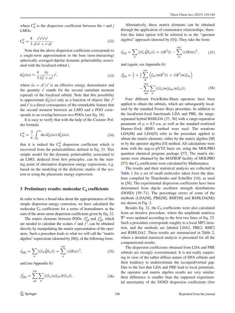
where C
ij
6 is the dispersion coeffi cient between the i and j
LMOs:
Note that the above dispersion coeffi cient corresponds to
a single-term approximation to the bare (non-interacting)
spherically averaged dipolar dynamic polarizability associated with the localized orbital i ,
where ω i = Δ i /s i is an effective energy denominator and
the quantity s i stands for the second cumulant moment
(spread) of the localized orbital. Note that this possibility
to approximate α i
0 (iω) only as a function of objects like f i
and s i is a direct consequence of the remarkable feature that
the second moment between an LMO and a POO corresponds to an overlap between two POOs (see Eq. 18 ).
It is easy to verify that with the help of the Casimir–Polder formula
that it is indeed the C
ij
6 dispersion coeffi cient which is
recovered from the polarizabilities defi ned in Eq. 33 . This
simple model for the dynamic polarizability associated to
an LMO, deduced from fi rst principles, can be the starting point of alternative dispersion energy expressions, e.g.
based on the modeling of the dielectric matrix of the system or using the plasmonic energy expression.
3 Preliminary results: molecular C 6 coeffi cients
In order to have a broad idea about the appropriateness of this
simple dispersion energy correction, we have calculated the
molecular C 6 coeffi cients for a series of homodimers as the
sum of the atom–atom dispersion coeffi cients given by Eq. 32 .
The matrix elements between POOs, S ii
αβ and f ii
αβ , which
are needed to calculate the scalars s i and f i , can be obtained
directly by manipulating the matrix representation of the operators. Such a procedure leads to what we will call the “matrix
algebra” expressions (denoted by [M]), of the following form:
and (see Appendix 6 ):
(32)
C
ij
6 =
8
3
s i s j s i s j
Δ i s j + s i Δ j .
(33)
α
i
0 (iω) ≈
4
3
ω i
ω 2
i + ω 2 s
i ,
(34)
C
ij
6 =
3
π
∞
0
dω α
i
0 (iω) α
j
0 (iω),
(35)
s
i
[M] =
α
i|ˆ r α ˆ
Qˆ r α |i =
virt
a
||i|ˆ r|a|
2 ,
(36)
f
i
[M] =
virt
ab
α
i|ˆ r α |af ab b|ˆ r α |i.
Alternatively, these matrix elements can be obtained
through the application of commutator relationships, therefore this latter option will be referred to as the “operator
algebra” approach (denoted by [O]). They take the form:
and (again, see Appendix 6 ):
Four different Fock/Kohn-Sham operators have been
applied to obtain the orbitals, which are subsequently localized by the standard Foster–Boys procedure. In addition to
the local/semi-local functionals LDA and PBE, the rangeseparated hybrid RSHLDA [ 37 , 56 ] with a range-separation
parameter of μ = 0.5 a.u. as well as the standard restricted
Hartree–Fock (RHF) method were used. The notations
LDA[M] and LDA[O] refer to the procedure applied to
obtain the matrix elements: either by the matrix algebra [M]
or by the operator algebra [O] method. All calculations were
done with the aug-cc-pVTZ basis set, using the MOLPRO
quantum chemical program package [ 57 ]. The matrix elements were obtained by the MATROP facility of MOLPRO
[ 57 ]; the C 6 coeffi cients were calculated by Mathematica.
The results and their statistical analysis are collected in
Table 1 for a set of small molecules taken from the database compiled by Tkatchenko and Scheffl er [ 16 ], as used
in [ 58 ]. The experimental dispersion coeffi cients have been
determined from dipole oscillator strength distributions
(DOSD) [ 59 – 71 ]. The percentage errors of some of the
methods (LDA[M], PBE[M], RHF[M] and RSHLDA[M])
are shown in Fig. 3 .
Besides Eq. 32 , the C 6 coeffi cients were also calculated
from an iterative procedure, where the amplitude matrices
T ij were updated according to the fi rst two lines of Eq. 23 .
Such a procedure corresponds roughly to a local MP2 iteration, and the methods are labeled LDA2, PBE2, RHF2
and RSHLDA2. These results are summarized in Table 2 ,
where a detailed statistical analysis is presented for all the
computational results.
The dispersion coeffi cients obtained from LDA and PBE
orbitals are strongly overestimated. It is not really surprising in view of the rather diffuse nature of DFA orbitals and
their tendency to underestimate the occupied/virtual gap.
Due to the fact that LDA and PBE lead to local potentials,
the operator and matrix algebra results are very similar:
their difference is smaller than the supposed experimental uncertainty of the DOSD dispersion coeffi cients (few
(37)
s
i
[O] =
α
i|ˆ r α ˆ
Qˆ r α |i = =i|ˆ r
2
|i −
occ
m
||i|ˆ r|m|
2 ,
(38)
f
i
[O] =
3
2 +
1
2
occ
m
f im m|ˆ r
2
|i + +i|ˆ r
2
|mf mi
−
occ
mn
α
i|ˆ r α |mf mn n|ˆ r α |i.
106
Reprinted from the journal
1 3
where C
ij
6 is the dispersion coeffi cient between the i and j
LMOs:
Note that the above dispersion coeffi cient corresponds to
a single-term approximation to the bare (non-interacting)
spherically averaged dipolar dynamic polarizability associated with the localized orbital i ,
where ω i = Δ i /s i is an effective energy denominator and
the quantity s i stands for the second cumulant moment
(spread) of the localized orbital. Note that this possibility
to approximate α i
0 (iω) only as a function of objects like f i
and s i is a direct consequence of the remarkable feature that
the second moment between an LMO and a POO corresponds to an overlap between two POOs (see Eq. 18 ).
It is easy to verify that with the help of the Casimir–Polder formula
that it is indeed the C
ij
6 dispersion coeffi cient which is
recovered from the polarizabilities defi ned in Eq. 33 . This
simple model for the dynamic polarizability associated to
an LMO, deduced from fi rst principles, can be the starting point of alternative dispersion energy expressions, e.g.
based on the modeling of the dielectric matrix of the system or using the plasmonic energy expression.
3 Preliminary results: molecular C 6 coeffi cients
In order to have a broad idea about the appropriateness of this
simple dispersion energy correction, we have calculated the
molecular C 6 coeffi cients for a series of homodimers as the
sum of the atom–atom dispersion coeffi cients given by Eq. 32 .
The matrix elements between POOs, S ii
αβ and f ii
αβ , which
are needed to calculate the scalars s i and f i , can be obtained
directly by manipulating the matrix representation of the operators. Such a procedure leads to what we will call the “matrix
algebra” expressions (denoted by [M]), of the following form:
and (see Appendix 6 ):
(32)
C
ij
6 =
8
3
s i s j s i s j
Δ i s j + s i Δ j .
(33)
α
i
0 (iω) ≈
4
3
ω i
ω 2
i + ω 2 s
i ,
(34)
C
ij
6 =
3
π
∞
0
dω α
i
0 (iω) α
j
0 (iω),
(35)
s
i
[M] =
α
i|ˆ r α ˆ
Qˆ r α |i =
virt
a
||i|ˆ r|a|
2 ,
(36)
f
i
[M] =
virt
ab
α
i|ˆ r α |af ab b|ˆ r α |i.
Alternatively, these matrix elements can be obtained
through the application of commutator relationships, therefore this latter option will be referred to as the “operator
algebra” approach (denoted by [O]). They take the form:
and (again, see Appendix 6 ):
Four different Fock/Kohn-Sham operators have been
applied to obtain the orbitals, which are subsequently localized by the standard Foster–Boys procedure. In addition to
the local/semi-local functionals LDA and PBE, the rangeseparated hybrid RSHLDA [ 37 , 56 ] with a range-separation
parameter of μ = 0.5 a.u. as well as the standard restricted
Hartree–Fock (RHF) method were used. The notations
LDA[M] and LDA[O] refer to the procedure applied to
obtain the matrix elements: either by the matrix algebra [M]
or by the operator algebra [O] method. All calculations were
done with the aug-cc-pVTZ basis set, using the MOLPRO
quantum chemical program package [ 57 ]. The matrix elements were obtained by the MATROP facility of MOLPRO
[ 57 ]; the C 6 coeffi cients were calculated by Mathematica.
The results and their statistical analysis are collected in
Table 1 for a set of small molecules taken from the database compiled by Tkatchenko and Scheffl er [ 16 ], as used
in [ 58 ]. The experimental dispersion coeffi cients have been
determined from dipole oscillator strength distributions
(DOSD) [ 59 – 71 ]. The percentage errors of some of the
methods (LDA[M], PBE[M], RHF[M] and RSHLDA[M])
are shown in Fig. 3 .
Besides Eq. 32 , the C 6 coeffi cients were also calculated
from an iterative procedure, where the amplitude matrices
T ij were updated according to the fi rst two lines of Eq. 23 .
Such a procedure corresponds roughly to a local MP2 iteration, and the methods are labeled LDA2, PBE2, RHF2
and RSHLDA2. These results are summarized in Table 2 ,
where a detailed statistical analysis is presented for all the
computational results.
The dispersion coeffi cients obtained from LDA and PBE
orbitals are strongly overestimated. It is not really surprising in view of the rather diffuse nature of DFA orbitals and
their tendency to underestimate the occupied/virtual gap.
Due to the fact that LDA and PBE lead to local potentials,
the operator and matrix algebra results are very similar:
their difference is smaller than the supposed experimental uncertainty of the DOSD dispersion coeffi cients (few
(37)
s
i
[O] =
α
i|ˆ r α ˆ
Qˆ r α |i = =i|ˆ r
2
|i −
occ
m
||i|ˆ r|m|
2 ,
(38)
f
i
[O] =
3
2 +
1
2
occ
m
f im m|ˆ r
2
|i + +i|ˆ r
2
|mf mi
−
occ
mn
α
i|ˆ r α |mf mn n|ˆ r α |i.
106
Reprinted from the journal