

Theor Chem Acc (2015) 134:148
1 3
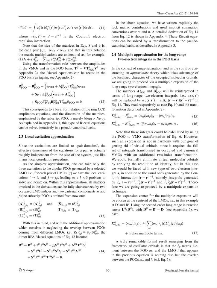
where w(r, r ) = |r − r| −1 is the Coulomb electron
repulsion interaction.
Note that the size of the matrices in Eqs. 8 and 9 is,
for each pair [ ij ], N virt × N virt and that in this notation
the matrix multiplications are understood as, for example:
(T(A + ))
ij
ab =
mc T im
ac A
mj
cb + T im
ac
mj
cb .
Using the transformation rule between the amplitudes
in the VMOs and in the POO basis, T ij = VT
ij
POO V † (see
Appendix 2 ), the Riccati equations can be recast in the
POO basis as (again, see Appendix 2 ):
This corresponds to a local formulation of the ring CCD
amplitudes equations, and the dimension of the matrices,
emphasized by the subscript POO, is merely N POO × N POO .
As explained in Appendix 3 , this type of Riccati equations
can be solved iteratively in a pseudo-canonical basis.
2.3 Local excitation approximation
Since the excitations are limited to “pair-domains”, the
effective dimension of the equations for a pair is actually
roughly independent from the size of the system, just like
in any local correlation procedure.
As the simplest approximation, one can take only the
three excitations to the dipolar POOs generated by a selected
LMO, i.e., for each pair of LMOs [ ij ] we have the local excitations i → i α and j → j β , leading to a 3 × 3 problem to
solve and iterate on. Within this approximation, all matrices
involved in the derivations can be fully characterized by two
occupied LMO indices and two cartesian components, α and
β (the subscript POO is omitted from now on):
With this in mind, and with the additional approximation
which consists in neglecting the overlap between POOs
coming from different LMOs, i.e., (S)
ij
αβ ≈ δ ij (S) ii
αβ , the
direct RPA Riccati equations of Eq. 12 become:
(11)
ij|ab =
φ
∗
i (r)φ
∗
j
r
w
r, r
φ a (r)φ b
r
drdr
,
(12)
R
ij
POO = B
ij
POO +
POO + A
im
POO
T
mj
POO S POO
+ S POO T
im
POO
POO + A
mj
POO
+ S POO T
im
POO B
mn
POO T
nj
POO S POO = 0.
(13)
(A)
ij
i α j β
≡ (A)
ij
αβ
and (S) i α j β ≡ (S)
ij
αβ
(B)
ij
i α j β
≡ (B)
ij
αβ
(f) i α j β ≡ (f)
ij
αβ
(T)
ij
i α j β
≡ (T)
ij
αβ
(14)
R
ij
= B
ij
+ f
ii T
ij S
jj
− f ii S
ii T
ij S
jj
+ A
im T
mj S
jj
+ S
ii T
ij f
jj
− S
ii T
ij S
jj f jj + S
ii T
im A
mj
+ S
ii T
im B
mn T
nj S
jj
= 0.
In the above equation, we have written explicitly the
fock matrix contributions and used implicit summation
conventions over m and n . A detailed derivation of Eq. 14
from Eq. 12 is shown in Appendix 4 . These Riccati equations can be solved by a transformation to the pseudocanonical basis, as described in Appendix 3 .
2.4 Multipole approximation for the long-range
two-electron integrals in the POO basis
In the context of range-separation, and in the spirit of constructing an approximate theory which takes advantage of
the localized character of the occupied molecular orbitals,
we are going to proceed via a multipole expansion of the
long-range two-electron integrals.
The matrices A
ij
POO and B
ij
POO will be reinterpreted in
terms of long-range two-electron integrals, i.e., w(r, r )
will be replaced by w lr (r, r ) = erf(μ|r − r|)|r − r| −1 in
Eq. 11 . They read respectively as (see Eq. 10 and the transformation described in Appendix 2 ):
Note that these integrals could be calculated by using
the POO to VMO transformation of Eq. 6 . However,
such an expression is not in harmony with our goal of
getting rid of virtual orbitals, since it requires the full
set of integrals transformed in occupied and canonical
VMOs with an additional two-index transformation.
We could formally eliminate virtual molecular orbitals
by applying the resolution of identity, but in this case
we would be faced with new type of two-electron integrals, in addition to the usual ones generated by the Coulomb interaction |r − r | −1 , namely integrals generated
by ˆ
r α |r − r | −1 , ˆ
r
β |r − r | −1 and ˆ
r α ˆ
r
β |r − r | −1 . Therefore we are going to proceed by a multipole expansion
technique.
The expansion center for the multipole expansion will
be chosen at the centroid of the LMOs, i.e., in this example
at D i and D j . Using the second-order long-range interaction
tensor L ij (D ij ), with D ij = D i − D j (see Appendix 5 ), we
have
A truly remarkable formal result emerging from the
framework of oscillator orbitals is that the ˆ
r γ matrix element between the POO m α and the LMO i that appears
in the previous equation is nothing else but the overlap
between the POOs m α and i γ (c.f. Eq. 5 ):
(15)
K
ij
m α n β
− J
ij
m α n β
= =m α j|in β lr − −m α j|n β i lr
(16)
K
ij
m α n β
− K
ij
m α n β
= =ij|m α n β lr − −ij|n β m α lr .
(17)
K
ij
m α n β
= =m α j|in β lr ≈
γ δ
m α |ˆ r γ |iL
ij
γ δ j|ˆ r δ |n β
+ higher multipole terms.
104
Reprinted from the journal
1 3
where w(r, r ) = |r − r| −1 is the Coulomb electron
repulsion interaction.
Note that the size of the matrices in Eqs. 8 and 9 is,
for each pair [ ij ], N virt × N virt and that in this notation
the matrix multiplications are understood as, for example:
(T(A + ))
ij
ab =
mc T im
ac A
mj
cb + T im
ac
mj
cb .
Using the transformation rule between the amplitudes
in the VMOs and in the POO basis, T ij = VT
ij
POO V † (see
Appendix 2 ), the Riccati equations can be recast in the
POO basis as (again, see Appendix 2 ):
This corresponds to a local formulation of the ring CCD
amplitudes equations, and the dimension of the matrices,
emphasized by the subscript POO, is merely N POO × N POO .
As explained in Appendix 3 , this type of Riccati equations
can be solved iteratively in a pseudo-canonical basis.
2.3 Local excitation approximation
Since the excitations are limited to “pair-domains”, the
effective dimension of the equations for a pair is actually
roughly independent from the size of the system, just like
in any local correlation procedure.
As the simplest approximation, one can take only the
three excitations to the dipolar POOs generated by a selected
LMO, i.e., for each pair of LMOs [ ij ] we have the local excitations i → i α and j → j β , leading to a 3 × 3 problem to
solve and iterate on. Within this approximation, all matrices
involved in the derivations can be fully characterized by two
occupied LMO indices and two cartesian components, α and
β (the subscript POO is omitted from now on):
With this in mind, and with the additional approximation
which consists in neglecting the overlap between POOs
coming from different LMOs, i.e., (S)
ij
αβ ≈ δ ij (S) ii
αβ , the
direct RPA Riccati equations of Eq. 12 become:
(11)
ij|ab =
φ
∗
i (r)φ
∗
j
r
w
r, r
φ a (r)φ b
r
drdr
,
(12)
R
ij
POO = B
ij
POO +
POO + A
im
POO
T
mj
POO S POO
+ S POO T
im
POO
POO + A
mj
POO
+ S POO T
im
POO B
mn
POO T
nj
POO S POO = 0.
(13)
(A)
ij
i α j β
≡ (A)
ij
αβ
and (S) i α j β ≡ (S)
ij
αβ
(B)
ij
i α j β
≡ (B)
ij
αβ
(f) i α j β ≡ (f)
ij
αβ
(T)
ij
i α j β
≡ (T)
ij
αβ
(14)
R
ij
= B
ij
+ f
ii T
ij S
jj
− f ii S
ii T
ij S
jj
+ A
im T
mj S
jj
+ S
ii T
ij f
jj
− S
ii T
ij S
jj f jj + S
ii T
im A
mj
+ S
ii T
im B
mn T
nj S
jj
= 0.
In the above equation, we have written explicitly the
fock matrix contributions and used implicit summation
conventions over m and n . A detailed derivation of Eq. 14
from Eq. 12 is shown in Appendix 4 . These Riccati equations can be solved by a transformation to the pseudocanonical basis, as described in Appendix 3 .
2.4 Multipole approximation for the long-range
two-electron integrals in the POO basis
In the context of range-separation, and in the spirit of constructing an approximate theory which takes advantage of
the localized character of the occupied molecular orbitals,
we are going to proceed via a multipole expansion of the
long-range two-electron integrals.
The matrices A
ij
POO and B
ij
POO will be reinterpreted in
terms of long-range two-electron integrals, i.e., w(r, r )
will be replaced by w lr (r, r ) = erf(μ|r − r|)|r − r| −1 in
Eq. 11 . They read respectively as (see Eq. 10 and the transformation described in Appendix 2 ):
Note that these integrals could be calculated by using
the POO to VMO transformation of Eq. 6 . However,
such an expression is not in harmony with our goal of
getting rid of virtual orbitals, since it requires the full
set of integrals transformed in occupied and canonical
VMOs with an additional two-index transformation.
We could formally eliminate virtual molecular orbitals
by applying the resolution of identity, but in this case
we would be faced with new type of two-electron integrals, in addition to the usual ones generated by the Coulomb interaction |r − r | −1 , namely integrals generated
by ˆ
r α |r − r | −1 , ˆ
r
β |r − r | −1 and ˆ
r α ˆ
r
β |r − r | −1 . Therefore we are going to proceed by a multipole expansion
technique.
The expansion center for the multipole expansion will
be chosen at the centroid of the LMOs, i.e., in this example
at D i and D j . Using the second-order long-range interaction
tensor L ij (D ij ), with D ij = D i − D j (see Appendix 5 ), we
have
A truly remarkable formal result emerging from the
framework of oscillator orbitals is that the ˆ
r γ matrix element between the POO m α and the LMO i that appears
in the previous equation is nothing else but the overlap
between the POOs m α and i γ (c.f. Eq. 5 ):
(15)
K
ij
m α n β
− J
ij
m α n β
= =m α j|in β lr − −m α j|n β i lr
(16)
K
ij
m α n β
− K
ij
m α n β
= =ij|m α n β lr − −ij|n β m α lr .
(17)
K
ij
m α n β
= =m α j|in β lr ≈
γ δ
m α |ˆ r γ |iL
ij
γ δ j|ˆ r δ |n β
+ higher multipole terms.
104
Reprinted from the journal