

Theor Chem Acc (2015) 134:148
1 3
where ˆ
f μ φ i = ˆ t + ˆ
v ne + ˆ
v H + ˆ
v
lr,μ
x,HF + ˆ
v
sr,μ
xc,DFA is the rangeseparated hybrid operator. In this expression ˆ t is the kinetic
energy, ˆ
v ne is the nuclear attraction, ˆ
v H is the full-range
Hartree, ˆ
v
lr,μ
x,HF is the long-range Hartree–Fock (non-local)
exchange, and ˆ
v
sr,μ
xc,DFA is the short-range exchange-correlation potential operator. The range-separation parameter, μ ,
defi ned below, cuts the electron repulsion terms to shortand long-range components. For μ = 0 one recovers the
full-range DFA, while for μ → ∞ one obtains the fullrange Hartree–Fock theory.
As outlined in the introduction, inspired by the original
idea suggested fi rst by Foster and Boys [ 24 ] and refi ned
later by Boys [ 26 ], we propose here to construct localized virtual orbitals by multiplying the localized occupied
orbital φ i (r) by solid spherical harmonics having their origin at the barycenter (centroid) of the localized occupied
orbital. According to Boys [ 26 ], this defi nition can be made
independent of the orientation of the coordinate system by
choosing local coordinate axes which are parallel to the
principal axes of the tensor of the moment of inertia of the
charge distribution φ ∗
i (r)φ i (r) (see Appendix 1 ).
In the following we are going to elaborate the theory for
the simplest case, when these oscillator orbitals are generated by fi rst-order solid spherical harmonic polynomials,
i.e., the i th LMO is multiplied by (ˆ r α − D i
α ) , where ˆ
r α is the
α = x, y, z component of the position operator and D i
α is a
component of the position vector pointing to the centroid
of the i th LMO, defi ned as D i
α = =φ i |ˆ r α |φ i . It is possible
to generate oscillator orbitals by higher order spherical harmonics too, which is left for forthcoming work. We denote
the POO by | ˜
φ i α , where the index i α refers to the fact that
the OO has been generated from the i th LMO by using the
ˆ
r α function. For the sake of the simplicity of the formulae,
the POOs will be expressed in the laboratory frame; the
expressions for the dipolar POOs in a local frame are
shown in the Appendix 1 . The POO reads in the laboratory
frame as
with ˆ
Q = ( ˆ
I −
occ
m |φ m φ m |), the projector onto the virtual space.
In Eq. 4 the “pure” (OO) component of the POO is
ˆ
r α |φ i , while the orthogonalization tails stem from the term
−
occ
m =i |φ m φ m |ˆ r α |φ i . In this sense the “locality” of the
OO is somewhat deteriorated, since we have contributions
from each of the other LMOs. At this point the Boys localization criterion will be at our advantage, since it ensures
that the sum of the off-diagonal elements of the x , y and z
operators taken between the occupied orbitals, and appearing in the orthogonalization tails, be minimized [ 55 ]. In this
sense, the Boys-localization scheme seems to be naturally
adapted for the construction of dipolar oscillator orbitals.
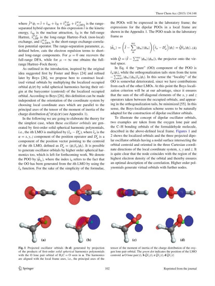
To illustrate the concept of dipolar oscillator orbitals,
two examples are taken from the oxygen lone pair and
the C–H bonding orbitals of the formaldehyde molecule,
described in the above-defi ned local frame. Figures 1 and
2 shows the localized orbitals and the three projected dipolar oscillator orbitals having a nodal surface intersecting the
orbital centroid and oriented in the three Cartesian coordinate directions of the local coordinate system, x , y and z . It
is quite clear that the node coincides with the region of the
highest electron density of the orbital and thereby ensures
an optimal description of the correlation. Higher order polynomials generate virtual orbitals with further nodes.
(4)
| ˜
φ i α =
ˆ
I −
occ
m
|φ m φ m |
ˆ
r α − D
i
α
|φ i = ˆ
Qˆ r α |φ i ,
Fig. 1 Projected oscillator orbitals ( b – d ) generated by projection
of the products of fi rst-order solid spherical harmonics polynomials
with the O lone pair orbital of H 2 C = O seen in a . The harmonics
are aligned with the local frame axes, i.e., the principal axes of the
tensor of the moment of inertia of the charge distribution of the oxygen lone pair orbital. The green dot indicates the position of the LMO
centroid. a O lone pair |i , b ˆ
Qˆ r x |i , c ˆ
Qˆ r y |i , d ˆ
Qˆ r z |i
102
Reprinted from the journal
1 3
where ˆ
f μ φ i = ˆ t + ˆ
v ne + ˆ
v H + ˆ
v
lr,μ
x,HF + ˆ
v
sr,μ
xc,DFA is the rangeseparated hybrid operator. In this expression ˆ t is the kinetic
energy, ˆ
v ne is the nuclear attraction, ˆ
v H is the full-range
Hartree, ˆ
v
lr,μ
x,HF is the long-range Hartree–Fock (non-local)
exchange, and ˆ
v
sr,μ
xc,DFA is the short-range exchange-correlation potential operator. The range-separation parameter, μ ,
defi ned below, cuts the electron repulsion terms to shortand long-range components. For μ = 0 one recovers the
full-range DFA, while for μ → ∞ one obtains the fullrange Hartree–Fock theory.
As outlined in the introduction, inspired by the original
idea suggested fi rst by Foster and Boys [ 24 ] and refi ned
later by Boys [ 26 ], we propose here to construct localized virtual orbitals by multiplying the localized occupied
orbital φ i (r) by solid spherical harmonics having their origin at the barycenter (centroid) of the localized occupied
orbital. According to Boys [ 26 ], this defi nition can be made
independent of the orientation of the coordinate system by
choosing local coordinate axes which are parallel to the
principal axes of the tensor of the moment of inertia of the
charge distribution φ ∗
i (r)φ i (r) (see Appendix 1 ).
In the following we are going to elaborate the theory for
the simplest case, when these oscillator orbitals are generated by fi rst-order solid spherical harmonic polynomials,
i.e., the i th LMO is multiplied by (ˆ r α − D i
α ) , where ˆ
r α is the
α = x, y, z component of the position operator and D i
α is a
component of the position vector pointing to the centroid
of the i th LMO, defi ned as D i
α = =φ i |ˆ r α |φ i . It is possible
to generate oscillator orbitals by higher order spherical harmonics too, which is left for forthcoming work. We denote
the POO by | ˜
φ i α , where the index i α refers to the fact that
the OO has been generated from the i th LMO by using the
ˆ
r α function. For the sake of the simplicity of the formulae,
the POOs will be expressed in the laboratory frame; the
expressions for the dipolar POOs in a local frame are
shown in the Appendix 1 . The POO reads in the laboratory
frame as
with ˆ
Q = ( ˆ
I −
occ
m |φ m φ m |), the projector onto the virtual space.
In Eq. 4 the “pure” (OO) component of the POO is
ˆ
r α |φ i , while the orthogonalization tails stem from the term
−
occ
m =i |φ m φ m |ˆ r α |φ i . In this sense the “locality” of the
OO is somewhat deteriorated, since we have contributions
from each of the other LMOs. At this point the Boys localization criterion will be at our advantage, since it ensures
that the sum of the off-diagonal elements of the x , y and z
operators taken between the occupied orbitals, and appearing in the orthogonalization tails, be minimized [ 55 ]. In this
sense, the Boys-localization scheme seems to be naturally
adapted for the construction of dipolar oscillator orbitals.
To illustrate the concept of dipolar oscillator orbitals,
two examples are taken from the oxygen lone pair and
the C–H bonding orbitals of the formaldehyde molecule,
described in the above-defi ned local frame. Figures 1 and
2 shows the localized orbitals and the three projected dipolar oscillator orbitals having a nodal surface intersecting the
orbital centroid and oriented in the three Cartesian coordinate directions of the local coordinate system, x , y and z . It
is quite clear that the node coincides with the region of the
highest electron density of the orbital and thereby ensures
an optimal description of the correlation. Higher order polynomials generate virtual orbitals with further nodes.
(4)
| ˜
φ i α =
ˆ
I −
occ
m
|φ m φ m |
ˆ
r α − D
i
α
|φ i = ˆ
Qˆ r α |φ i ,
Fig. 1 Projected oscillator orbitals ( b – d ) generated by projection
of the products of fi rst-order solid spherical harmonics polynomials
with the O lone pair orbital of H 2 C = O seen in a . The harmonics
are aligned with the local frame axes, i.e., the principal axes of the
tensor of the moment of inertia of the charge distribution of the oxygen lone pair orbital. The green dot indicates the position of the LMO
centroid. a O lone pair |i , b ˆ
Qˆ r x |i , c ˆ
Qˆ r y |i , d ˆ
Qˆ r z |i
102
Reprinted from the journal