

After that, we go back to (37) for a new step with U
0,αα defined in (38). When
δ tresh1 ! ΔU
! αα
) δ tresh2 , the iterative procedure is resumed by the help of the
conjugated gradient technique described by Pople et al. [81]. It is not required in
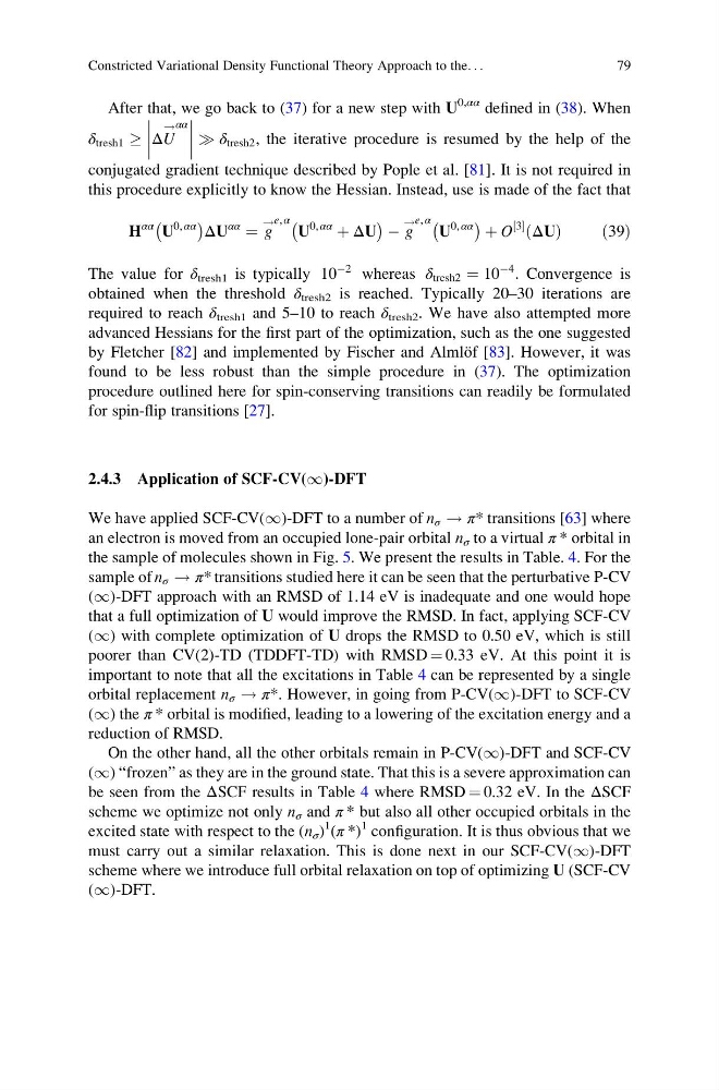
this procedure explicitly to know the Hessian. Instead, use is made of the fact that
H
αα U
0, αα
À
Á
ΔU
αα
¼ g
! e, α
U
0, αα
þ ΔU
À
Á À g
! e, α
U
0, αα
À
Á þ O
3
½
ΔU
ð Þ
ð39Þ
The value for δ tresh1 is typically 10
À2 whereas δ tresh2 ¼ 10
À4 . Convergence is
obtained when the threshold δ tresh2 is reached. Typically 20–30 iterations are
required to reach δ tresh1 and 5–10 to reach δ tresh2 . We have also attempted more
advanced Hessians for the first part of the optimization, such as the one suggested
by Fletcher [82] and implemented by Fischer and Almlo ¨f [83]. However, it was
found to be less robust than the simple procedure in (37). The optimization
procedure outlined here for spin-conserving transitions can readily be formulated
for spin-flip transitions [27].
2.4.3 Application of SCF-CV(1)-DFT
We have applied SCF-CV(1)-DFT to a number of n σ ! π* transitions [63] where
an electron is moved from an occupied lone-pair orbital n σ to a virtual π * orbital in
the sample of molecules shown in Fig. 5. We present the results in Table. 4. For the
sample of n σ ! π* transitions studied here it can be seen that the perturbative P-CV
(1)-DFT approach with an RMSD of 1.14 eV is inadequate and one would hope
that a full optimization of U would improve the RMSD. In fact, applying SCF-CV
(1) with complete optimization of U drops the RMSD to 0.50 eV, which is still
poorer than CV(2)-TD (TDDFT-TD) with RMSD ¼ 0.33 eV. At this point it is
important to note that all the excitations in Table 4 can be represented by a single
orbital replacement n σ ! π*. However, in going from P-CV(1)-DFT to SCF-CV
(1) the π * orbital is modified, leading to a lowering of the excitation energy and a
reduction of RMSD.
On the other hand, all the other orbitals remain in P-CV(1)-DFT and SCF-CV
(1) “frozen” as they are in the ground state. That this is a severe approximation can
be seen from the ΔSCF results in Table 4 where RMSD ¼ 0.32 eV. In the ΔSCF
scheme we optimize not only n σ and π * but also all other occupied orbitals in the
excited state with respect to the (n σ )
1
(π *)
1 configuration. It is thus obvious that we
must carry out a similar relaxation. This is done next in our SCF-CV(1)-DFT
scheme where we introduce full orbital relaxation on top of optimizing U (SCF-CV
(1)-DFT.
Constricted Variational Density Functional Theory Approach to the. . .
79
0,αα defined in (38). When
δ tresh1 ! ΔU
! αα
) δ tresh2 , the iterative procedure is resumed by the help of the
conjugated gradient technique described by Pople et al. [81]. It is not required in
this procedure explicitly to know the Hessian. Instead, use is made of the fact that
H
αα U
0, αα
À
Á
ΔU
αα
¼ g
! e, α
U
0, αα
þ ΔU
À
Á À g
! e, α
U
0, αα
À
Á þ O
3
½
ΔU
ð Þ
ð39Þ
The value for δ tresh1 is typically 10
À2 whereas δ tresh2 ¼ 10
À4 . Convergence is
obtained when the threshold δ tresh2 is reached. Typically 20–30 iterations are
required to reach δ tresh1 and 5–10 to reach δ tresh2 . We have also attempted more
advanced Hessians for the first part of the optimization, such as the one suggested
by Fletcher [82] and implemented by Fischer and Almlo ¨f [83]. However, it was
found to be less robust than the simple procedure in (37). The optimization
procedure outlined here for spin-conserving transitions can readily be formulated
for spin-flip transitions [27].
2.4.3 Application of SCF-CV(1)-DFT
We have applied SCF-CV(1)-DFT to a number of n σ ! π* transitions [63] where
an electron is moved from an occupied lone-pair orbital n σ to a virtual π * orbital in
the sample of molecules shown in Fig. 5. We present the results in Table. 4. For the
sample of n σ ! π* transitions studied here it can be seen that the perturbative P-CV
(1)-DFT approach with an RMSD of 1.14 eV is inadequate and one would hope
that a full optimization of U would improve the RMSD. In fact, applying SCF-CV
(1) with complete optimization of U drops the RMSD to 0.50 eV, which is still
poorer than CV(2)-TD (TDDFT-TD) with RMSD ¼ 0.33 eV. At this point it is
important to note that all the excitations in Table 4 can be represented by a single
orbital replacement n σ ! π*. However, in going from P-CV(1)-DFT to SCF-CV
(1) the π * orbital is modified, leading to a lowering of the excitation energy and a
reduction of RMSD.
On the other hand, all the other orbitals remain in P-CV(1)-DFT and SCF-CV
(1) “frozen” as they are in the ground state. That this is a severe approximation can
be seen from the ΔSCF results in Table 4 where RMSD ¼ 0.32 eV. In the ΔSCF
scheme we optimize not only n σ and π * but also all other occupied orbitals in the
excited state with respect to the (n σ )
1
(π *)
1 configuration. It is thus obvious that we
must carry out a similar relaxation. This is done next in our SCF-CV(1)-DFT
scheme where we introduce full orbital relaxation on top of optimizing U (SCF-CV
(1)-DFT.
Constricted Variational Density Functional Theory Approach to the. . .
79