

g
! α, e
ai U
0, αα
À
Á ¼
dΔE M
dΔU
αα
ai
0
¼
δΔE M
δρ α
0
dΔρ
α
dΔU
αα
ai
0
¼
ð
F KS
Â
ρ
0
=2 þ 1=2Δρ
α
M , ρ
0
=2
à ∂Δρ
α
M
dU
αα
ai
0
dv 1 ;
ð35Þ
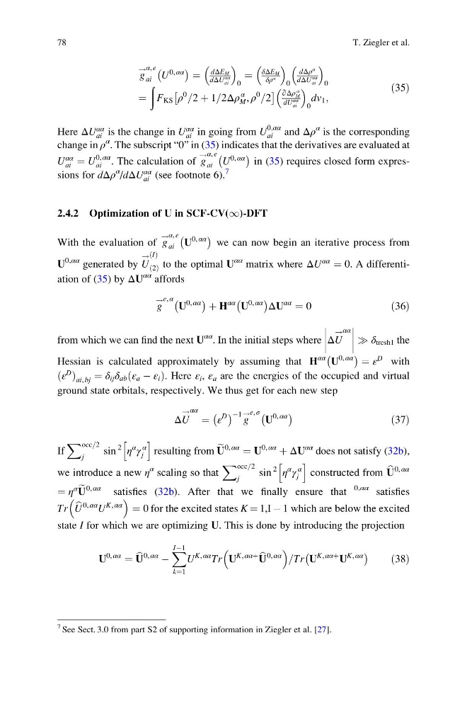
Here ΔU
αα
ai is the change in U
αα
ai in going from U
0;αα
ai
and Δρ
α is the corresponding
change in ρ
α . The subscript “0” in (35) indicates that the derivatives are evaluated at
U
αα
ai ¼ U
0, αα
ai . The calculation of g
! α, e
ai U
0, αα
À
Á
in (35) requires closed form expressions for dΔρ
α
/dΔU
αα
ai (see footnote 6).
7
2.4.2 Optimization of U in SCF-CV(1)-DFT
With the evaluation of g
! α, e
ai U
0, αα
À
Á
we can now begin an iterative process from
U
0,αα generated by U
! I
ð Þ
2
ð Þ to the optimal U
αα matrix where ΔU
αα
¼ 0. A differentiation of (35) by ΔU
αα affords
g
! e, α
U
0, αα
À
Á þ H
αα U
0, αα
À
Á ΔU
αα
¼ 0
ð36Þ
from which we can find the next U
αα . In the initial steps where ΔU
! αα
) δ tresh1 the
Hessian is calculated approximately by assuming that H
αα U
0, αα
À
Á ¼ ε
D with
ε
D
ð Þ ai, bj ¼ δ ij δ ab ε a À ε i
ð
Þ. Here ε i , ε a are the energies of the occupied and virtual
ground state orbitals, respectively. We thus get for each new step
ΔU
! αα
¼ ε
D
À Á À1 g
! e, σ
U
0, αα
À
Á
ð37Þ
If
X occ=2
j
sin
2
η
α
γ
α
j
h
i
resulting from e
U
0, αα
¼ U
0, αα
þ ΔU
αα does not satisfy (32b),
we introduce a new η
α scaling so that
X occ=2
j
sin
2
η
α
γ
α
j
h
i
constructed from b
U
0, αα
¼ η
α e
U
0, αα
satisfies (32b). After that we finally ensure that
0,αα satisfies
Tr b
U
0, αα U
K, αα
¼ 0 for the excited states K ¼ 1,I À 1 which are below the excited
state I for which we are optimizing U. This is done by introducing the projection
U
0, αα
¼ b
U
0, αα
À
X IÀ1
k¼1
U
K, αα Tr U
K, ααþ b
U
0, αα
=Tr U
K, ααþ U
K, αα
À
Á
ð38Þ
7 See Sect. 3.0 from part S2 of supporting information in Ziegler et al. [27].
78
T. Ziegler et al.
! α, e
ai U
0, αα
À
Á ¼
dΔE M
dΔU
αα
ai
0
¼
δΔE M
δρ α
0
dΔρ
α
dΔU
αα
ai
0
¼
ð
F KS
Â
ρ
0
=2 þ 1=2Δρ
α
M , ρ
0
=2
à ∂Δρ
α
M
dU
αα
ai
0
dv 1 ;
ð35Þ
Here ΔU
αα
ai is the change in U
αα
ai in going from U
0;αα
ai
and Δρ
α is the corresponding
change in ρ
α . The subscript “0” in (35) indicates that the derivatives are evaluated at
U
αα
ai ¼ U
0, αα
ai . The calculation of g
! α, e
ai U
0, αα
À
Á
in (35) requires closed form expressions for dΔρ
α
/dΔU
αα
ai (see footnote 6).
7
2.4.2 Optimization of U in SCF-CV(1)-DFT
With the evaluation of g
! α, e
ai U
0, αα
À
Á
we can now begin an iterative process from
U
0,αα generated by U
! I
ð Þ
2
ð Þ to the optimal U
αα matrix where ΔU
αα
¼ 0. A differentiation of (35) by ΔU
αα affords
g
! e, α
U
0, αα
À
Á þ H
αα U
0, αα
À
Á ΔU
αα
¼ 0
ð36Þ
from which we can find the next U
αα . In the initial steps where ΔU
! αα
) δ tresh1 the
Hessian is calculated approximately by assuming that H
αα U
0, αα
À
Á ¼ ε
D with
ε
D
ð Þ ai, bj ¼ δ ij δ ab ε a À ε i
ð
Þ. Here ε i , ε a are the energies of the occupied and virtual
ground state orbitals, respectively. We thus get for each new step
ΔU
! αα
¼ ε
D
À Á À1 g
! e, σ
U
0, αα
À
Á
ð37Þ
If
X occ=2
j
sin
2
η
α
γ
α
j
h
i
resulting from e
U
0, αα
¼ U
0, αα
þ ΔU
αα does not satisfy (32b),
we introduce a new η
α scaling so that
X occ=2
j
sin
2
η
α
γ
α
j
h
i
constructed from b
U
0, αα
¼ η
α e
U
0, αα
satisfies (32b). After that we finally ensure that
0,αα satisfies
Tr b
U
0, αα U
K, αα
¼ 0 for the excited states K ¼ 1,I À 1 which are below the excited
state I for which we are optimizing U. This is done by introducing the projection
U
0, αα
¼ b
U
0, αα
À
X IÀ1
k¼1
U
K, αα Tr U
K, ααþ b
U
0, αα
=Tr U
K, ααþ U
K, αα
À
Á
ð38Þ
7 See Sect. 3.0 from part S2 of supporting information in Ziegler et al. [27].
78
T. Ziegler et al.