

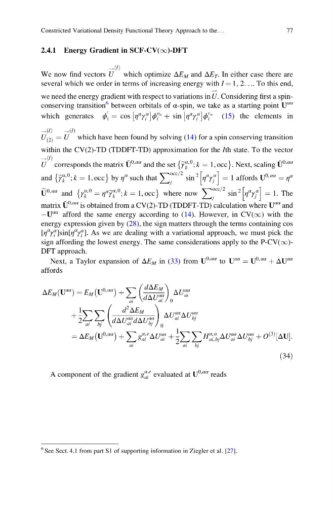
2.4.1 Energy Gradient in SCF-CV(1)-DFT
We now find vectors U
! I
ð Þ
which optimize ΔE M and ΔE T . In either case there are
several which we order in terms of increasing energy with I ¼ 1, 2. . .. To this end,
we need the energy gradient with respect to variations in U
!
. Considering first a spinconserving transition
6 between orbitals of α-spin, we take as a starting point U
αα
which generates ϕ
0
i ¼ cos η
α
γ
α
i
Â
Ã
ϕ
o α
i þ sin η
α
γ
α
i
Â
à ϕ
v α
i
(15) the elements in
U
! I
ð Þ
2
ð Þ ¼ U
! I
ð Þ
which have been found by solving (14) for a spin conserving transition
within the CV(2)-TD (TDDFT-TD) approximation for the Ith state. To the vector
U
! I
ð Þ
corresponds the matrix U ˜ 0,αα and the set e γ
α, 0
k ; k ¼ 1, occ
È
É
. Next, scaling U ˜ 0,αα
and e γ
α, 0
k ; k ¼ 1, occ
È
É
by η
α such that
X occ=2
j
sin
2
η
α
γ
α
j
h
i
¼ 1 affords U
0, αα
¼ η
α
e
U
0, αα and γ
α, 0
k ¼ η
α
e γ
α, 0
k ; k ¼ 1, occ
È
É
where now
X occ=2
j
sin
2
η
α
γ
α
j
h
i
¼ 1. The
matrix U ˜ 0,αα is obtained from a CV(2)-TD (TDDFT-TD) calculation where U
αα and
ÀU
αα afford the same energy according to (14). However, in CV(1) with the
energy expression given by (28), the sign matters through the terms containing cos
[η
α
γ
α
i ]sin[η
α
γ
α
i ]. As we are dealing with a variational approach, we must pick the
sign affording the lowest energy. The same considerations apply to the P-CV(1)DFT approach.
Next, a Taylor expansion of ΔE M in (33) from U
0,αα to U
αα
¼ U
0, αα
þ ΔU
αα
affords
ΔE M U
αα
ð
Þ¼ E M U
0, αα
À
Á þ
X
ai
dΔE M
dΔU
αα
ai
0
ΔU
αα
ai
þ
1
2
X
ai
X
bj
d
2
ΔE M
dΔU
αα
ai dΔU
αα
bj
!
0
ΔU
αα
ai ΔU
αα
bj
¼ ΔE M U
0, αα
À
Á þ
X
ai
g
α, e
ai ΔU
αα
ai þ
1
2
X
ai
X
bj
H
α, α
ai, bj ΔU
αα
ai ΔU
αα
bj þ O
3
ð Þ
ΔU
½ :
ð34Þ
A component of the gradient g
α;e
ai evaluated at U
0,αα reads
6 See Sect. 4.1 from part S1 of supporting information in Ziegler et al. [27].
Constricted Variational Density Functional Theory Approach to the. . .
77
We now find vectors U
! I
ð Þ
which optimize ΔE M and ΔE T . In either case there are
several which we order in terms of increasing energy with I ¼ 1, 2. . .. To this end,
we need the energy gradient with respect to variations in U
!
. Considering first a spinconserving transition
6 between orbitals of α-spin, we take as a starting point U
αα
which generates ϕ
0
i ¼ cos η
α
γ
α
i
Â
Ã
ϕ
o α
i þ sin η
α
γ
α
i
Â
à ϕ
v α
i
(15) the elements in
U
! I
ð Þ
2
ð Þ ¼ U
! I
ð Þ
which have been found by solving (14) for a spin conserving transition
within the CV(2)-TD (TDDFT-TD) approximation for the Ith state. To the vector
U
! I
ð Þ
corresponds the matrix U ˜ 0,αα and the set e γ
α, 0
k ; k ¼ 1, occ
È
É
. Next, scaling U ˜ 0,αα
and e γ
α, 0
k ; k ¼ 1, occ
È
É
by η
α such that
X occ=2
j
sin
2
η
α
γ
α
j
h
i
¼ 1 affords U
0, αα
¼ η
α
e
U
0, αα and γ
α, 0
k ¼ η
α
e γ
α, 0
k ; k ¼ 1, occ
È
É
where now
X occ=2
j
sin
2
η
α
γ
α
j
h
i
¼ 1. The
matrix U ˜ 0,αα is obtained from a CV(2)-TD (TDDFT-TD) calculation where U
αα and
ÀU
αα afford the same energy according to (14). However, in CV(1) with the
energy expression given by (28), the sign matters through the terms containing cos
[η
α
γ
α
i ]sin[η
α
γ
α
i ]. As we are dealing with a variational approach, we must pick the
sign affording the lowest energy. The same considerations apply to the P-CV(1)DFT approach.
Next, a Taylor expansion of ΔE M in (33) from U
0,αα to U
αα
¼ U
0, αα
þ ΔU
αα
affords
ΔE M U
αα
ð
Þ¼ E M U
0, αα
À
Á þ
X
ai
dΔE M
dΔU
αα
ai
0
ΔU
αα
ai
þ
1
2
X
ai
X
bj
d
2
ΔE M
dΔU
αα
ai dΔU
αα
bj
!
0
ΔU
αα
ai ΔU
αα
bj
¼ ΔE M U
0, αα
À
Á þ
X
ai
g
α, e
ai ΔU
αα
ai þ
1
2
X
ai
X
bj
H
α, α
ai, bj ΔU
αα
ai ΔU
αα
bj þ O
3
ð Þ
ΔU
½ :
ð34Þ
A component of the gradient g
α;e
ai evaluated at U
0,αα reads
6 See Sect. 4.1 from part S1 of supporting information in Ziegler et al. [27].
Constricted Variational Density Functional Theory Approach to the. . .
77