

K
KS XC
ð Þ
ru,tq
¼
1
2
ð
ϕ
*
r r 1
ð Þϕ u r 1
ð Þϕ t r 1
ð Þϕ
*
q r 1
ð Þ
h
i 1
2
δ
2 E XC
δ
2
ρ α
þ
δ
2 E XC
δ
2
ρ β
À 2
δ
2 E XC
δρ α δρ α
!
ρ 0 ;s 0
ð
Þ
2
4
3
5 dr 1
¼ K
KS,XC
ru,tq À K
KS,XC
rt,uq
ð12Þ
where K
KS,XC
ru,tq ,K
KS,XC
rt,uq
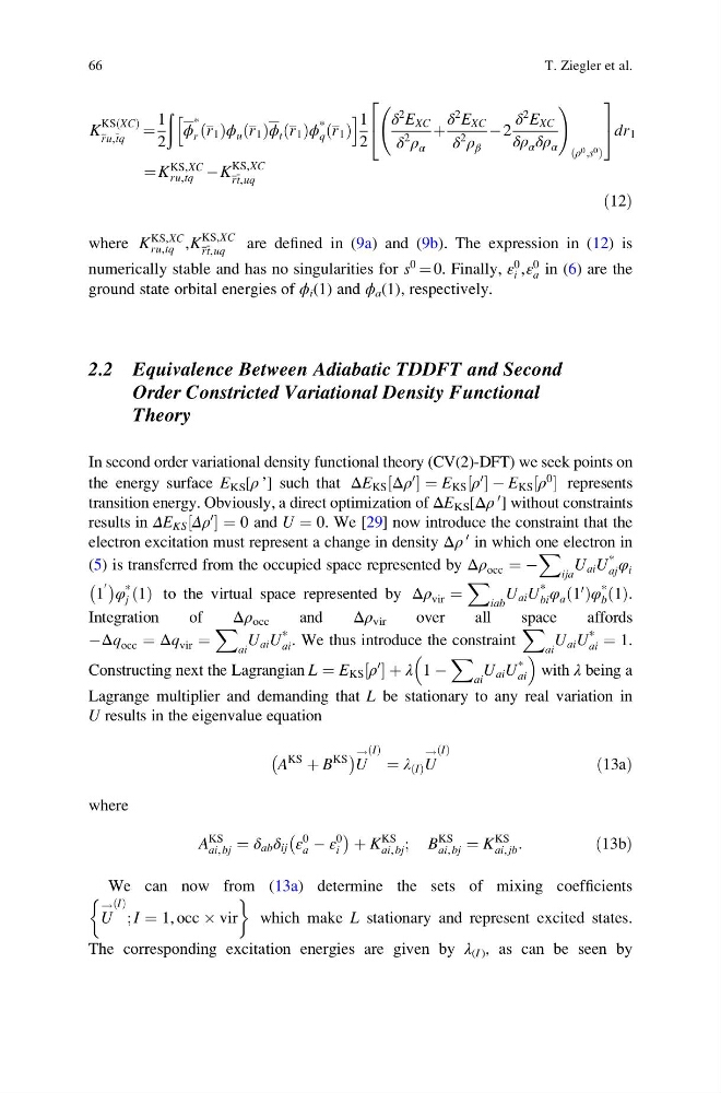
are defined in (9a) and (9b). The expression in (12) is
numerically stable and has no singularities for s
0
¼ 0. Finally, ε
0
i ,ε
0
a in (6) are the
ground state orbital energies of ϕ i (1) and ϕ a (1), respectively.
2.2 Equivalence Between Adiabatic TDDFT and Second
Order Constricted Variational Density Functional
Theory
In second order variational density functional theory (CV(2)-DFT) we seek points on
the energy surface E KS [ρ ’] such that ΔE KS Δρ
0
½ ¼ E KS ρ
0
½ À E KS ρ
0
½ represents
transition energy. Obviously, a direct optimization of ΔE KS [Δρ
0 ] without constraints
results in ΔE KS Δρ
0
½ ¼ 0 and U ¼ 0. We [29] now introduce the constraint that the
electron excitation must represent a change in density Δρ
0 in which one electron in
(5) is transferred from the occupied space represented by Δρ occ ¼ À
X
ija
U ai U
*
aj φ i
1
0
À Á φ
*
j 1
ð Þ to the virtual space represented by Δρ vir ¼
X
iab
U ai U
*
bi φ a 1
0
ð Þφ
*
b 1
ð Þ.
Integration
of
Δρ occ
and
Δρ vir
over
all
space
affords
ÀΔq occ ¼ Δq vir ¼
X
ai
U ai U
*
ai . We thus introduce the constraint
X
ai
U ai U
*
ai ¼ 1.
Constructing next the Lagrangian L ¼ E KS ρ
0
½ þ λ 1 À
X
ai
U ai U
*
ai
with λ being a
Lagrange multiplier and demanding that L be stationary to any real variation in
U results in the eigenvalue equation
A
KS
þ B
KS
À
Á
U
! I
ð Þ
¼ λ I
ð Þ U
! I
ð Þ
ð13aÞ
where
A
KS
ai, bj ¼ δ ab δ ij ε
0
a À ε
0
i
À
Á þ K
KS
ai, bj ; B
KS
ai, bj ¼ K
KS
ai, jb :
ð13bÞ
We can now from (13a) determine the sets of mixing coefficients
U
! I
ð Þ
; I ¼ 1, occ  vir
&
'
which make L stationary and represent excited states.
The corresponding excitation energies are given by λ (I ) , as can be seen by
66
T. Ziegler et al.
KS XC
ð Þ
ru,tq
¼
1
2
ð
ϕ
*
r r 1
ð Þϕ u r 1
ð Þϕ t r 1
ð Þϕ
*
q r 1
ð Þ
h
i 1
2
δ
2 E XC
δ
2
ρ α
þ
δ
2 E XC
δ
2
ρ β
À 2
δ
2 E XC
δρ α δρ α
!
ρ 0 ;s 0
ð
Þ
2
4
3
5 dr 1
¼ K
KS,XC
ru,tq À K
KS,XC
rt,uq
ð12Þ
where K
KS,XC
ru,tq ,K
KS,XC
rt,uq
are defined in (9a) and (9b). The expression in (12) is
numerically stable and has no singularities for s
0
¼ 0. Finally, ε
0
i ,ε
0
a in (6) are the
ground state orbital energies of ϕ i (1) and ϕ a (1), respectively.
2.2 Equivalence Between Adiabatic TDDFT and Second
Order Constricted Variational Density Functional
Theory
In second order variational density functional theory (CV(2)-DFT) we seek points on
the energy surface E KS [ρ ’] such that ΔE KS Δρ
0
½ ¼ E KS ρ
0
½ À E KS ρ
0
½ represents
transition energy. Obviously, a direct optimization of ΔE KS [Δρ
0 ] without constraints
results in ΔE KS Δρ
0
½ ¼ 0 and U ¼ 0. We [29] now introduce the constraint that the
electron excitation must represent a change in density Δρ
0 in which one electron in
(5) is transferred from the occupied space represented by Δρ occ ¼ À
X
ija
U ai U
*
aj φ i
1
0
À Á φ
*
j 1
ð Þ to the virtual space represented by Δρ vir ¼
X
iab
U ai U
*
bi φ a 1
0
ð Þφ
*
b 1
ð Þ.
Integration
of
Δρ occ
and
Δρ vir
over
all
space
affords
ÀΔq occ ¼ Δq vir ¼
X
ai
U ai U
*
ai . We thus introduce the constraint
X
ai
U ai U
*
ai ¼ 1.
Constructing next the Lagrangian L ¼ E KS ρ
0
½ þ λ 1 À
X
ai
U ai U
*
ai
with λ being a
Lagrange multiplier and demanding that L be stationary to any real variation in
U results in the eigenvalue equation
A
KS
þ B
KS
À
Á
U
! I
ð Þ
¼ λ I
ð Þ U
! I
ð Þ
ð13aÞ
where
A
KS
ai, bj ¼ δ ab δ ij ε
0
a À ε
0
i
À
Á þ K
KS
ai, bj ; B
KS
ai, bj ¼ K
KS
ai, jb :
ð13bÞ
We can now from (13a) determine the sets of mixing coefficients
U
! I
ð Þ
; I ¼ 1, occ  vir
&
'
which make L stationary and represent excited states.
The corresponding excitation energies are given by λ (I ) , as can be seen by
66
T. Ziegler et al.