

procedure gives rise to the nth order CV-DFT scheme designated as CV(n)-DFT
[26–28].
We start this review by an outline of the CV(n)-DFT theory. This framework
enables us to identify ATDDFT and ΔSCF as special cases of the CV(n)-DFT
scheme with ATDDFT being equivalent to CV(2)-DFT [29, 62] whereas ΔSCF
corresponds to CV(1)-DFT under the simplifying assumption that the excited state
under investigation can be described by a single orbital replacement i ! a
ð
Þ [27,
44]. The theoretical exposition is followed by first assessing the general performance of CV(n)-DFT in connection with applications to n ! π* [26–67] and
π ! π* [27] transitions in organic molecules. After that we demonstrate that CV
(n)-DFT is able to deal with a number of transitions where the performance of
ATDDFT based on local and hybrid functionals is problematic. These transitions
involve π ! π* excitations in organic dyes [64, 65] as well as π ! π* transitions in
charge transfer adducts [30] and Rydberg excitations for atoms and small molecules
[66]. We finally discuss future directions for the development and application of the
CV(n)-DFT scheme.
2 Constricted Variational Density Functional Theory
We have recently introduced a variational approach based on density functional
theory for the description of excited states [29, 31]. In this constricted variational
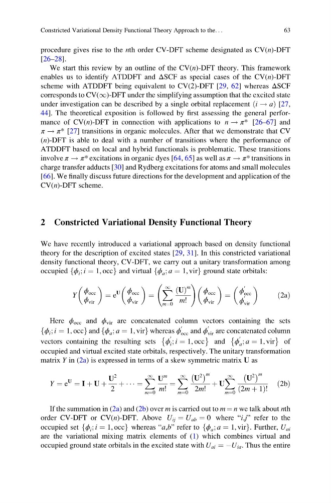
density functional theory, CV-DFT, we carry out a unitary transformation among
occupied ϕ i ; i ¼ 1, occ
f
gand virtual ϕ a ; a ¼ 1, vir
f
gground state orbitals:
Y
ϕ occ
ϕ vir
¼ e
U ϕ occ
ϕ vir
¼
X 1
m¼0
U
ð Þ
m
m!
!
ϕ occ
ϕ vir
¼
ϕ
0
occ
ϕ
0
vir
ð2aÞ
Here ϕ occ and ϕ vir are concatenated column vectors containing the sets
ϕ i ; i ¼ 1, occ
f
g and ϕ a ; a ¼ 1, vir
f
g whereas ϕ
0
occ and ϕ
0
vir are concatenated column
vectors containing the resulting sets ϕ
0
i ; i ¼ 1, occ
È
É
and ϕ
0
a ; a ¼ 1, vir
È
É
of
occupied and virtual excited state orbitals, respectively. The unitary transformation
matrix Y in (2a) is expressed in terms of a skew symmetric matrix U as
Y ¼ e
U
¼ I þ U þ
U
2
2
þ Á Á Á ¼
X 1
m¼0
U
m
m!
¼
X 1
m¼0
U
2
À Á m
2m!
þ U
X 1
m¼0
U
2
À Á m
2m þ 1
ð
Þ!
ð2bÞ
If the summation in (2a) and (2b) over m is carried out to m ¼ n we talk about nth
order CV-DFT or CV(n)-DFT. Above U ij ¼ U ab ¼ 0 where “i,j” refer to the
occupied set ϕ i ; i ¼ 1, occ
f
gwhereas “a,b” refer to ϕ a ; a ¼ 1, vir
f
g . Further, U ai
are the variational mixing matrix elements of (1) which combines virtual and
occupied ground state orbitals in the excited state with U ai ¼ ÀU ia . Thus the entire
Constricted Variational Density Functional Theory Approach to the. . .
63
[26–28].
We start this review by an outline of the CV(n)-DFT theory. This framework
enables us to identify ATDDFT and ΔSCF as special cases of the CV(n)-DFT
scheme with ATDDFT being equivalent to CV(2)-DFT [29, 62] whereas ΔSCF
corresponds to CV(1)-DFT under the simplifying assumption that the excited state
under investigation can be described by a single orbital replacement i ! a
ð
Þ [27,
44]. The theoretical exposition is followed by first assessing the general performance of CV(n)-DFT in connection with applications to n ! π* [26–67] and
π ! π* [27] transitions in organic molecules. After that we demonstrate that CV
(n)-DFT is able to deal with a number of transitions where the performance of
ATDDFT based on local and hybrid functionals is problematic. These transitions
involve π ! π* excitations in organic dyes [64, 65] as well as π ! π* transitions in
charge transfer adducts [30] and Rydberg excitations for atoms and small molecules
[66]. We finally discuss future directions for the development and application of the
CV(n)-DFT scheme.
2 Constricted Variational Density Functional Theory
We have recently introduced a variational approach based on density functional
theory for the description of excited states [29, 31]. In this constricted variational
density functional theory, CV-DFT, we carry out a unitary transformation among
occupied ϕ i ; i ¼ 1, occ
f
gand virtual ϕ a ; a ¼ 1, vir
f
gground state orbitals:
Y
ϕ occ
ϕ vir
¼ e
U ϕ occ
ϕ vir
¼
X 1
m¼0
U
ð Þ
m
m!
!
ϕ occ
ϕ vir
¼
ϕ
0
occ
ϕ
0
vir
ð2aÞ
Here ϕ occ and ϕ vir are concatenated column vectors containing the sets
ϕ i ; i ¼ 1, occ
f
g and ϕ a ; a ¼ 1, vir
f
g whereas ϕ
0
occ and ϕ
0
vir are concatenated column
vectors containing the resulting sets ϕ
0
i ; i ¼ 1, occ
È
É
and ϕ
0
a ; a ¼ 1, vir
È
É
of
occupied and virtual excited state orbitals, respectively. The unitary transformation
matrix Y in (2a) is expressed in terms of a skew symmetric matrix U as
Y ¼ e
U
¼ I þ U þ
U
2
2
þ Á Á Á ¼
X 1
m¼0
U
m
m!
¼
X 1
m¼0
U
2
À Á m
2m!
þ U
X 1
m¼0
U
2
À Á m
2m þ 1
ð
Þ!
ð2bÞ
If the summation in (2a) and (2b) over m is carried out to m ¼ n we talk about nth
order CV-DFT or CV(n)-DFT. Above U ij ¼ U ab ¼ 0 where “i,j” refer to the
occupied set ϕ i ; i ¼ 1, occ
f
gwhereas “a,b” refer to ϕ a ; a ¼ 1, vir
f
g . Further, U ai
are the variational mixing matrix elements of (1) which combines virtual and
occupied ground state orbitals in the excited state with U ai ¼ ÀU ia . Thus the entire
Constricted Variational Density Functional Theory Approach to the. . .
63