

^
p
{
^
q
T
{
1
0
ð Þ ¼ T
{
1
T
{
1
;
ð156Þ
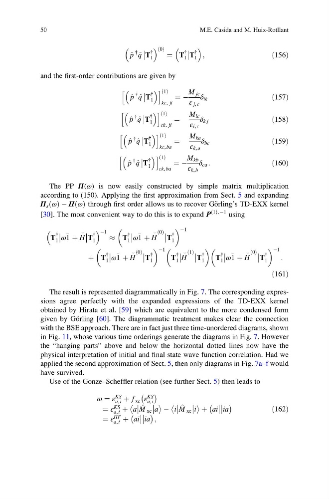
and the first-order contributions are given by
^
p
{
^
q
T
{
1
h
i 1
ð Þ
kc, ji
¼ À
M jc
ε j, c
δ ik
ð157Þ
^
p
{
^
q
T
{
1
h
i 1
ð Þ
ck, ji
¼
M ic
ε i, c
δ k j
ð158Þ
^
p
{
^
q
T
{
1
h
i 1
ð Þ
kc, ba
¼
M ka
ε k, a
δ bc
ð159Þ
^
p
{
^
q
T
{
1
h
i 1
ð Þ
ck, ba
¼ À
M kb
ε k, b
δ ca :
ð160Þ
The PP Π(ω) is now easily constructed by simple matrix multiplication
according to (150). Applying the first approximation from Sect. 5 and expanding
Π s ω
ð Þ À Π ω
ð Þ through first order allows us to recover G€ orling’s TD-EXX kernel
[30]. The most convenient way to do this is to expand P
1
ð Þ, À1 using
T
{
1
ω1
^ þ H
^
T
{
1
À1 % T
{
1
ω1
^ þ H
^ 0
ð Þ
T
{
1
À1
þ T
{
1
ω1
^ þ H
^ 0
ð Þ
T
{
1
À1
T
{
1
H
^ 1
ð Þ
T
{
1
T
{
1
ω1
^ þ H
^ 0
ð Þ
T
{
1
À1
:
ð161Þ
The result is represented diagrammatically in Fig. 7. The corresponding expressions agree perfectly with the expanded expressions of the TD-EXX kernel
obtained by Hirata et al. [59] which are equivalent to the more condensed form
given by G€ orling [60]. The diagrammatic treatment makes clear the connection
with the BSE approach. There are in fact just three time-unordered diagrams, shown
in Fig. 11, whose various time orderings generate the diagrams in Fig. 7. However
the “hanging parts” above and below the horizontal dotted lines now have the
physical interpretation of initial and final state wave function correlation. Had we
applied the second approximation of Sect. 5, then only diagrams in Fig. 7a–f would
have survived.
Use of the Gonze–Scheffler relation (see further Sect. 5) then leads to
ω ¼ ε
KS
a, i þ f xc ε
KS
a, i
À Á
¼ ε
KS
a, i þ a
^
M xc
a
À i
^
M xc
i
þ ai
ia
À
Á
¼ ε
HF
a, i þ ai
ia
À
Á ;
ð162Þ
50
M.E. Casida and M. Huix-Rotllant
p
{
^
q
T
{
1
0
ð Þ ¼ T
{
1
T
{
1
;
ð156Þ
and the first-order contributions are given by
^
p
{
^
q
T
{
1
h
i 1
ð Þ
kc, ji
¼ À
M jc
ε j, c
δ ik
ð157Þ
^
p
{
^
q
T
{
1
h
i 1
ð Þ
ck, ji
¼
M ic
ε i, c
δ k j
ð158Þ
^
p
{
^
q
T
{
1
h
i 1
ð Þ
kc, ba
¼
M ka
ε k, a
δ bc
ð159Þ
^
p
{
^
q
T
{
1
h
i 1
ð Þ
ck, ba
¼ À
M kb
ε k, b
δ ca :
ð160Þ
The PP Π(ω) is now easily constructed by simple matrix multiplication
according to (150). Applying the first approximation from Sect. 5 and expanding
Π s ω
ð Þ À Π ω
ð Þ through first order allows us to recover G€ orling’s TD-EXX kernel
[30]. The most convenient way to do this is to expand P
1
ð Þ, À1 using
T
{
1
ω1
^ þ H
^
T
{
1
À1 % T
{
1
ω1
^ þ H
^ 0
ð Þ
T
{
1
À1
þ T
{
1
ω1
^ þ H
^ 0
ð Þ
T
{
1
À1
T
{
1
H
^ 1
ð Þ
T
{
1
T
{
1
ω1
^ þ H
^ 0
ð Þ
T
{
1
À1
:
ð161Þ
The result is represented diagrammatically in Fig. 7. The corresponding expressions agree perfectly with the expanded expressions of the TD-EXX kernel
obtained by Hirata et al. [59] which are equivalent to the more condensed form
given by G€ orling [60]. The diagrammatic treatment makes clear the connection
with the BSE approach. There are in fact just three time-unordered diagrams, shown
in Fig. 11, whose various time orderings generate the diagrams in Fig. 7. However
the “hanging parts” above and below the horizontal dotted lines now have the
physical interpretation of initial and final state wave function correlation. Had we
applied the second approximation of Sect. 5, then only diagrams in Fig. 7a–f would
have survived.
Use of the Gonze–Scheffler relation (see further Sect. 5) then leads to
ω ¼ ε
KS
a, i þ f xc ε
KS
a, i
À Á
¼ ε
KS
a, i þ a
^
M xc
a
À i
^
M xc
i
þ ai
ia
À
Á
¼ ε
HF
a, i þ ai
ia
À
Á ;
ð162Þ
50
M.E. Casida and M. Huix-Rotllant