

ψ j 1
ð Þψ
*
b 1
ð Þ
ω À ε b, j
ψ b
v x ε b, j
À Á
ψ j
D
E
%
ψ j 1
ð Þψ
*
b 1
ð Þ
ω À ε b, j
ψ b
^
Σ x
ψ j
D
E
;
ð131Þ
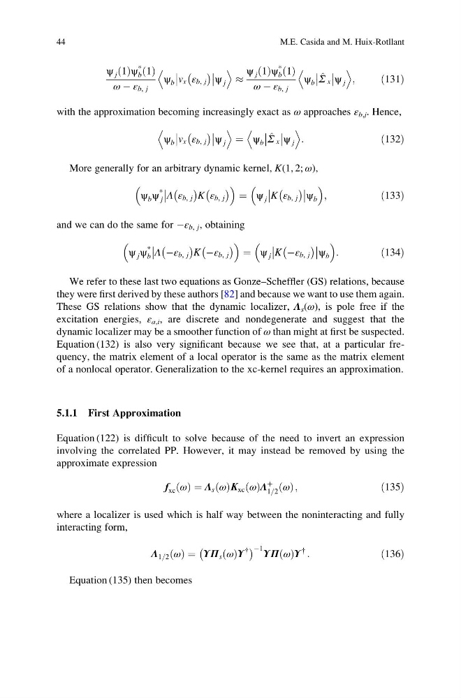
with the approximation becoming increasingly exact as ω approaches ε b,j . Hence,
ψ b
v x ε b, j
À Á
ψ j
D
E
¼ ψ b
^
Σ x
ψ j
D
E
:
ð132Þ
More generally for an arbitrary dynamic kernel, K(1, 2; ω),
ψ b ψ
*
j
Λ ε b, j
À Á
K ε b, j
À Á
¼ ψ j
K ε b, j
À Á
ψ b
;
ð133Þ
and we can do the same for Àε b, j , obtaining
ψ j ψ
*
b
Λ Àε b, j
À
Á
K Àε b, j
À
Á
¼ ψ j
K Àε b, j
À
Á
ψ b
:
ð134Þ
We refer to these last two equations as Gonze–Scheffler (GS) relations, because
they were first derived by these authors [82] and because we want to use them again.
These GS relations show that the dynamic localizer, Λ s (ω), is pole free if the
excitation energies, ε a,i , are discrete and nondegenerate and suggest that the
dynamic localizer may be a smoother function of ω than might at first be suspected.
Equation (132) is also very significant because we see that, at a particular frequency, the matrix element of a local operator is the same as the matrix element
of a nonlocal operator. Generalization to the xc-kernel requires an approximation.
5.1.1 First Approximation
Equation (122) is difficult to solve because of the need to invert an expression
involving the correlated PP. However, it may instead be removed by using the
approximate expression
f xc ω
ð Þ ¼ Λ s ω
ð ÞK xc ω
ð ÞΛ
þ
1=2 ω
ð Þ;
ð135Þ
where a localizer is used which is half way between the noninteracting and fully
interacting form,
Λ 1=2 ω
ð Þ ¼ ΥΠ s ω
ð ÞΥ
{
À
Á À1 ΥΠ ω
ð ÞΥ
{
:
ð136Þ
Equation (135) then becomes
44
M.E. Casida and M. Huix-Rotllant
ð Þψ
*
b 1
ð Þ
ω À ε b, j
ψ b
v x ε b, j
À Á
ψ j
D
E
%
ψ j 1
ð Þψ
*
b 1
ð Þ
ω À ε b, j
ψ b
^
Σ x
ψ j
D
E
;
ð131Þ
with the approximation becoming increasingly exact as ω approaches ε b,j . Hence,
ψ b
v x ε b, j
À Á
ψ j
D
E
¼ ψ b
^
Σ x
ψ j
D
E
:
ð132Þ
More generally for an arbitrary dynamic kernel, K(1, 2; ω),
ψ b ψ
*
j
Λ ε b, j
À Á
K ε b, j
À Á
¼ ψ j
K ε b, j
À Á
ψ b
;
ð133Þ
and we can do the same for Àε b, j , obtaining
ψ j ψ
*
b
Λ Àε b, j
À
Á
K Àε b, j
À
Á
¼ ψ j
K Àε b, j
À
Á
ψ b
:
ð134Þ
We refer to these last two equations as Gonze–Scheffler (GS) relations, because
they were first derived by these authors [82] and because we want to use them again.
These GS relations show that the dynamic localizer, Λ s (ω), is pole free if the
excitation energies, ε a,i , are discrete and nondegenerate and suggest that the
dynamic localizer may be a smoother function of ω than might at first be suspected.
Equation (132) is also very significant because we see that, at a particular frequency, the matrix element of a local operator is the same as the matrix element
of a nonlocal operator. Generalization to the xc-kernel requires an approximation.
5.1.1 First Approximation
Equation (122) is difficult to solve because of the need to invert an expression
involving the correlated PP. However, it may instead be removed by using the
approximate expression
f xc ω
ð Þ ¼ Λ s ω
ð ÞK xc ω
ð ÞΛ
þ
1=2 ω
ð Þ;
ð135Þ
where a localizer is used which is half way between the noninteracting and fully
interacting form,
Λ 1=2 ω
ð Þ ¼ ΥΠ s ω
ð ÞΥ
{
À
Á À1 ΥΠ ω
ð ÞΥ
{
:
ð136Þ
Equation (135) then becomes
44
M.E. Casida and M. Huix-Rotllant