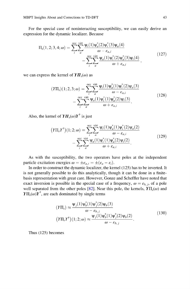
For the special case of noninteracting susceptibility, we can easily derive an
expression for the dynamic localizer. Because
Π s 1; 2; 3; 4; ω
ð
Þ¼
X occ
i
X virt
a
ψ i 1
ð Þψ
*
a 2
ð Þψ
*
i 3
ð Þψ a 4
ð Þ
ω À ε a, i
À
X occ
i
X virt
a
ψ a 1
ð Þψ
*
i 2
ð Þψ
*
a 3
ð Þψ i 4
ð Þ
ω þ ε a, i
;
ð127Þ
we can express the kernel of ΥΠ s (ω) as
Υ Π s
ð
Þ 1; 2; 3; ω
ð
Þ¼
X occ
i
X virt
a
ψ i 1
ð Þψ
*
a 1
ð Þψ
*
i 2
ð Þψ a 3
ð Þ
ω À ε a, i
À
X occ
i
X virt
a
ψ a 1
ð Þψ
*
i 1
ð Þψ
*
a 2
ð Þψ i 3
ð Þ
ω þ ε a, i
:
ð128Þ
Also, the kernel of ΥΠ s (ω)Υ
{ is just
Υ Π s Υ
{
À
Á
1; 2; ω
ð
Þ¼
X occ
i
X virt
a
ψ i 1
ð Þψ
*
a 1
ð Þψ
*
i 2
ð Þψ a 2
ð Þ
ω À ε a, i
À
X occ
i
X virt
a
ψ a 1
ð Þψ
*
i 1
ð Þψ
*
a 2
ð Þψ i 2
ð Þ
ω þ ε a, i
:
ð129Þ
As with the susceptibility, the two operators have poles at the independent
particle excitation energies ω ¼ Æε a, i ¼ Æ ε a À ε i
ð
Þ.
In order to construct the dynamic localizer, the kernel (125) has to be inverted. It
is not generally possible to do this analytically, though it can be done in a finitebasis representation with great care. However, Gonze and Scheffler have noted that
exact inversion is possible in the special case of a frequency, ω ¼ ε b, j , of a pole
well separated from the other poles [82]. Near this pole, the kernels, ΥΠ s (ω) and
ΥΠ s (ω)Υ
{ , are each dominated by single terms
Υ Π s
ð
Þ %
ψ j 1
ð Þψ
*
b 1
ð Þψ
*
j 2
ð Þψ b 3
ð Þ
ω À ε b, j
Υ Π s Υ
{
À
Á
1; 2; ω
ð
Þ%
ψ j 1
ð Þψ
*
b 1
ð Þψ
*
j 2
ð Þψ b 2
ð Þ
ω À ε b, j
:
ð130Þ
Thus (125) becomes
MBPT Insights About and Corrections to TD-DFT
43