

ð
ΥΠ s t 1 À t 3
ð
ÞΥ
{
f xc t 3 À t 4
ð
ÞΥΠ t 4 À t 2
ð
ÞΥ
{ dt 3 dt 4 ¼
ð
ΥΠ s t 1 À t 3
ð
ÞΥ
{
K xc t 3 À t 4
ð
ÞΥΠ t 4 À t 2
ð
Þdt 3 dt 4 ;
ð120Þ
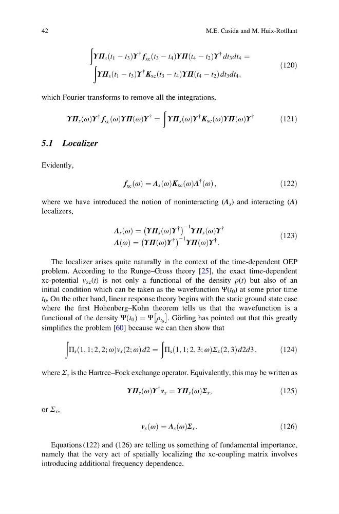
which Fourier transforms to remove all the integrations,
ΥΠ s ω
ð ÞΥ
{
f xc ω
ð ÞΥΠ ω
ð ÞΥ
{
¼
ð
ΥΠ s ω
ð ÞΥ
{
K xc ω
ð ÞΥΠ ω
ð ÞΥ
{
ð121Þ
5.1 Localizer
Evidently,
f xc ω
ð Þ ¼ Λ s ω
ð ÞK xc ω
ð ÞΛ
{
ω
ð Þ;
ð122Þ
where we have introduced the notion of noninteracting (Λ s ) and interacting (Λ)
localizers,
Λ s ω
ð Þ ¼ ΥΠ s ω
ð ÞΥ
{
À
Á À1 ΥΠ s ω
ð ÞΥ
{
Λ ω
ð Þ ¼ ΥΠ ω
ð ÞΥ
{
À
Á À1 ΥΠ ω
ð ÞΥ
{
:
ð123Þ
The localizer arises quite naturally in the context of the time-dependent OEP
problem. According to the Runge–Gross theory [25], the exact time-dependent
xc-potential v xc (t) is not only a functional of the density ρ(t) but also of an
initial condition which can be taken as the wavefunction Ψ(t 0 ) at some prior time
t 0 . On the other hand, linear response theory begins with the static ground state case
where the first Hohenberg–Kohn theorem tells us that the wavefunction is a
functional of the density Ψ t 0
ð Þ ¼ Ψ ρ t 0
 Ã
. G€ orling has pointed out that this greatly
simplifies the problem [60] because we can then show that
ð
Π s 1; 1; 2; 2; ω
ð
Þ v x 2; ω
ð
Þd2 ¼
ð
Π s 1; 1; 2; 3; ω
ð
Þ Σ x 2; 3
ð Þd2d3 ;
ð124Þ
where Σ x is the Hartree–Fock exchange operator. Equivalently, this may be written as
ΥΠ s ω
ð ÞΥ
{
v x ¼ ΥΠ s ω
ð ÞΣ x ;
ð125Þ
or Σ x ,
v x ω
ð Þ ¼ Λ s ω
ð ÞΣ x :
ð126Þ
Equations (122) and (126) are telling us something of fundamental importance,
namely that the very act of spatially localizing the xc-coupling matrix involves
introducing additional frequency dependence.
42
M.E. Casida and M. Huix-Rotllant
ΥΠ s t 1 À t 3
ð
ÞΥ
{
f xc t 3 À t 4
ð
ÞΥΠ t 4 À t 2
ð
ÞΥ
{ dt 3 dt 4 ¼
ð
ΥΠ s t 1 À t 3
ð
ÞΥ
{
K xc t 3 À t 4
ð
ÞΥΠ t 4 À t 2
ð
Þdt 3 dt 4 ;
ð120Þ
which Fourier transforms to remove all the integrations,
ΥΠ s ω
ð ÞΥ
{
f xc ω
ð ÞΥΠ ω
ð ÞΥ
{
¼
ð
ΥΠ s ω
ð ÞΥ
{
K xc ω
ð ÞΥΠ ω
ð ÞΥ
{
ð121Þ
5.1 Localizer
Evidently,
f xc ω
ð Þ ¼ Λ s ω
ð ÞK xc ω
ð ÞΛ
{
ω
ð Þ;
ð122Þ
where we have introduced the notion of noninteracting (Λ s ) and interacting (Λ)
localizers,
Λ s ω
ð Þ ¼ ΥΠ s ω
ð ÞΥ
{
À
Á À1 ΥΠ s ω
ð ÞΥ
{
Λ ω
ð Þ ¼ ΥΠ ω
ð ÞΥ
{
À
Á À1 ΥΠ ω
ð ÞΥ
{
:
ð123Þ
The localizer arises quite naturally in the context of the time-dependent OEP
problem. According to the Runge–Gross theory [25], the exact time-dependent
xc-potential v xc (t) is not only a functional of the density ρ(t) but also of an
initial condition which can be taken as the wavefunction Ψ(t 0 ) at some prior time
t 0 . On the other hand, linear response theory begins with the static ground state case
where the first Hohenberg–Kohn theorem tells us that the wavefunction is a
functional of the density Ψ t 0
ð Þ ¼ Ψ ρ t 0
 Ã
. G€ orling has pointed out that this greatly
simplifies the problem [60] because we can then show that
ð
Π s 1; 1; 2; 2; ω
ð
Þ v x 2; ω
ð
Þd2 ¼
ð
Π s 1; 1; 2; 3; ω
ð
Þ Σ x 2; 3
ð Þd2d3 ;
ð124Þ
where Σ x is the Hartree–Fock exchange operator. Equivalently, this may be written as
ΥΠ s ω
ð ÞΥ
{
v x ¼ ΥΠ s ω
ð ÞΣ x ;
ð125Þ
or Σ x ,
v x ω
ð Þ ¼ Λ s ω
ð ÞΣ x :
ð126Þ
Equations (122) and (126) are telling us something of fundamental importance,
namely that the very act of spatially localizing the xc-coupling matrix involves
introducing additional frequency dependence.
42
M.E. Casida and M. Huix-Rotllant