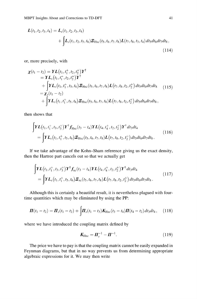
L t 1 ; t 2 ; t 3 ; t 4
ð
Þ¼L s t 1 ; t 2 ; t 3 ; t 4
ð
Þ
þ
ð
L s t 1 ; t 2 ; t 5 ; t 6
ð
Þ Ξ Hxc t 5 ; t 6 ; t 7 ; t 8
ð
Þ L t 7 ; t 8 ; t 3 ; t 4
ð
Þ dt 5 dt 6 dt 7 dt 8 ;
ð114Þ
or, more precisely, with
χ t 1 À t 2
ð
Þ¼ΥL t 1 ; t
þ
1 ; t 2 ; t
þ
2
À
Á Υ
{
¼ ΥL s t 1 ; t
þ
1 ; t 2 ; t
þ
2
À
Á Υ
{
þ
ð
ΥL s t 1 ; t
þ
1 ; t 5 ; t 6
À
Á Ξ Hxc t 5 ; t 6 ; t 7 ; t 8
ð
Þ L t 7 ; t 8 ; t 2 ; t
þ
2
À
Á
dt 5 dt 6 dt 7 dt 8
¼ χ s t 1 À t 2
ð
Þ
þ
ð
ΥL s t 1 ; t
þ
1 ; t 5 ; t 6
À
Á Ξ Hxc t 5 ; t 6 ; t 7 ; t 8
ð
Þ L t 7 ; t 8 ; t 2 ; t
þ
2
À
Á
dt 5 dt 6 dt 7 dt 8 ;
ð115Þ
then shows that
ð
ΥL t 1 ; t
þ
1 ; t 3 ; t
þ
3
À
Á Υ
{
f Hxc t 3 À t 4
ð
ÞΥL t 4 ; t
þ
4 ; t 2 ; t
þ
2
À
Á Υ
{ dt 3 dt 4
¼
ð
ΥL s t 1 ; t
þ
1 ; t 5 ; t 6
À
Á
Ξ Hxc t 5 ; t 6 ; t 7 ; t 8
ð
Þ L t 7 ; t 8 ; t 2 ; t
þ
2
À
Á
dt 5 dt 6 dt 7 dt 8 :
ð116Þ
If we take advantage of the Kohn–Sham reference giving us the exact density,
then the Hartree part cancels out so that we actually get
ð
ΥL t 1 ; t
þ
1 ; t 3 ; t
þ
3
À
Á Υ
{
f xc t 3 À t 4
ð
ÞΥL t 4 ; t
þ
4 ; t 2 ; t
þ
2
À
Á Υ
{ dt 3 dt 4
¼
ð
ΥL s t 1 ; t
þ
1 ; t 5 ; t 6
À
Á Ξ xc t 5 ; t 6 ; t 7 ; t 8
ð
Þ L t 7 ; t 8 ; t 2 ; t
þ
2
À
Á
dt 5 dt 6 dt 7 dt 8 :
ð117Þ
Although this is certainly a beautiful result, it is nevertheless plagued with fourtime quantities which may be eliminated by using the PP:
Π t 1 À t 2
ð
Þ¼Π s t 1 À t 2
ð
Þþ
ð
Π s t 1 À t 3
ð
ÞK Hxc t 3 À t 4
ð
ÞΠ t 4 À t 2
ð
Þdt 3 dt 4 ; ð118Þ
where we have introduced the coupling matrix defined by
K Hxc ¼ Π
À1
s À Π
À1
:
ð119Þ
The price we have to pay is that the coupling matrix cannot be easily expanded in
Feynman diagrams, but that in no way prevents us from determining appropriate
algebraic expressions for it. We may then write
MBPT Insights About and Corrections to TD-DFT
41