

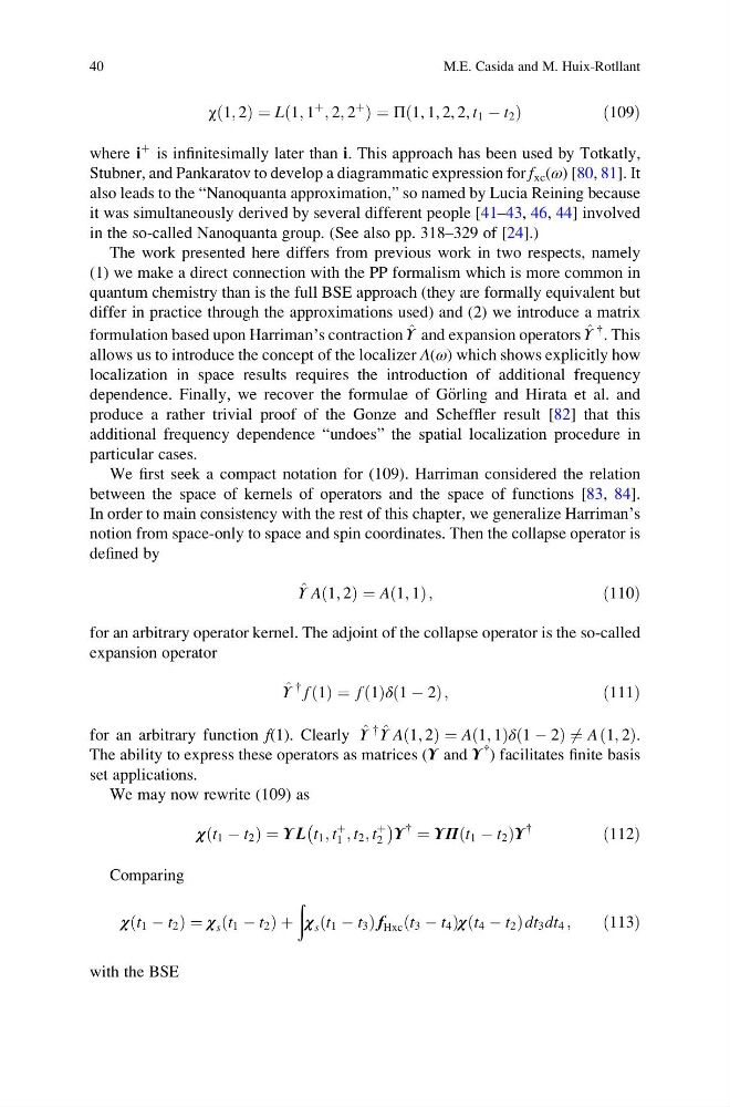
χ 1; 2
ð Þ ¼ L 1; 1
þ
; 2; 2
þ
ð
Þ¼Π 1, 1, 2, 2, t 1 À t 2
ð
Þ
ð 109Þ
where i
þ is infinitesimally later than i. This approach has been used by Totkatly,
Stubner, and Pankaratov to develop a diagrammatic expression for f xc (ω) [80, 81]. It
also leads to the “Nanoquanta approximation,” so named by Lucia Reining because
it was simultaneously derived by several different people [41–43, 46, 44] involved
in the so-called Nanoquanta group. (See also pp. 318–329 of [24].)
The work presented here differs from previous work in two respects, namely
(1) we make a direct connection with the PP formalism which is more common in
quantum chemistry than is the full BSE approach (they are formally equivalent but
differ in practice through the approximations used) and (2) we introduce a matrix
formulation based upon Harriman’s contraction ^
Υ and expansion operators ^
Υ
{ . This
allows us to introduce the concept of the localizer Λ(ω) which shows explicitly how
localization in space results requires the introduction of additional frequency
dependence. Finally, we recover the formulae of G€ orling and Hirata et al. and
produce a rather trivial proof of the Gonze and Scheffler result [82] that this
additional frequency dependence “undoes” the spatial localization procedure in
particular cases.
We first seek a compact notation for (109). Harriman considered the relation
between the space of kernels of operators and the space of functions [83, 84].
In order to main consistency with the rest of this chapter, we generalize Harriman’s
notion from space-only to space and spin coordinates. Then the collapse operator is
defined by
^
Υ A 1; 2
ð Þ ¼ A 1; 1
ð Þ;
ð110Þ
for an arbitrary operator kernel. The adjoint of the collapse operator is the so-called
expansion operator
^
Υ
{ f 1
ð Þ ¼ f 1
ð Þδ 1 À 2
ð
Þ;
ð111Þ
for an arbitrary function f(1). Clearly ^
Υ
{ ^
Υ A 1; 2
ð Þ ¼ A 1; 1
ð Þδ 1 À 2
ð
Þ6 ¼ A 1; 2
ð Þ.
The ability to express these operators as matrices (Υ and Υ
{ ) facilitates finite basis
set applications.
We may now rewrite (109) as
χ t 1 À t 2
ð
Þ¼ΥL t 1 ; t
þ
1 ; t 2 ; t
þ
2
À
Á Υ
{
¼ ΥΠ t 1 À t 2
ð
ÞΥ
{
ð112Þ
Comparing
χ t 1 À t 2
ð
Þ¼χ s t 1 À t 2
ð
Þþ
ð
χ s t 1 À t 3
ð
Þf Hxc t 3 À t 4
ð
Þχ t 4 À t 2
ð
Þdt 3 dt 4 ;
ð113Þ
with the BSE
40
M.E. Casida and M. Huix-Rotllant
ð Þ ¼ L 1; 1
þ
; 2; 2
þ
ð
Þ¼Π 1, 1, 2, 2, t 1 À t 2
ð
Þ
ð 109Þ
where i
þ is infinitesimally later than i. This approach has been used by Totkatly,
Stubner, and Pankaratov to develop a diagrammatic expression for f xc (ω) [80, 81]. It
also leads to the “Nanoquanta approximation,” so named by Lucia Reining because
it was simultaneously derived by several different people [41–43, 46, 44] involved
in the so-called Nanoquanta group. (See also pp. 318–329 of [24].)
The work presented here differs from previous work in two respects, namely
(1) we make a direct connection with the PP formalism which is more common in
quantum chemistry than is the full BSE approach (they are formally equivalent but
differ in practice through the approximations used) and (2) we introduce a matrix
formulation based upon Harriman’s contraction ^
Υ and expansion operators ^
Υ
{ . This
allows us to introduce the concept of the localizer Λ(ω) which shows explicitly how
localization in space results requires the introduction of additional frequency
dependence. Finally, we recover the formulae of G€ orling and Hirata et al. and
produce a rather trivial proof of the Gonze and Scheffler result [82] that this
additional frequency dependence “undoes” the spatial localization procedure in
particular cases.
We first seek a compact notation for (109). Harriman considered the relation
between the space of kernels of operators and the space of functions [83, 84].
In order to main consistency with the rest of this chapter, we generalize Harriman’s
notion from space-only to space and spin coordinates. Then the collapse operator is
defined by
^
Υ A 1; 2
ð Þ ¼ A 1; 1
ð Þ;
ð110Þ
for an arbitrary operator kernel. The adjoint of the collapse operator is the so-called
expansion operator
^
Υ
{ f 1
ð Þ ¼ f 1
ð Þδ 1 À 2
ð
Þ;
ð111Þ
for an arbitrary function f(1). Clearly ^
Υ
{ ^
Υ A 1; 2
ð Þ ¼ A 1; 1
ð Þδ 1 À 2
ð
Þ6 ¼ A 1; 2
ð Þ.
The ability to express these operators as matrices (Υ and Υ
{ ) facilitates finite basis
set applications.
We may now rewrite (109) as
χ t 1 À t 2
ð
Þ¼ΥL t 1 ; t
þ
1 ; t 2 ; t
þ
2
À
Á Υ
{
¼ ΥΠ t 1 À t 2
ð
ÞΥ
{
ð112Þ
Comparing
χ t 1 À t 2
ð
Þ¼χ s t 1 À t 2
ð
Þþ
ð
χ s t 1 À t 3
ð
Þf Hxc t 3 À t 4
ð
Þχ t 4 À t 2
ð
Þdt 3 dt 4 ;
ð113Þ
with the BSE
40
M.E. Casida and M. Huix-Rotllant