

at a somewhat higher, by ca. 0.4–0.8 eV, energy level than MRCISD. This difference may likely be caused by a somewhat stiffer C–C bond predicted by the DFT
calculations. This can be asserted from the x 1 vectors in Fig. 9, which describes a
C–C bond stretching combined with the C–C–O bending motion: there is a notably
greater degree of bond stretching in the MRCISD vector. As can be seen from
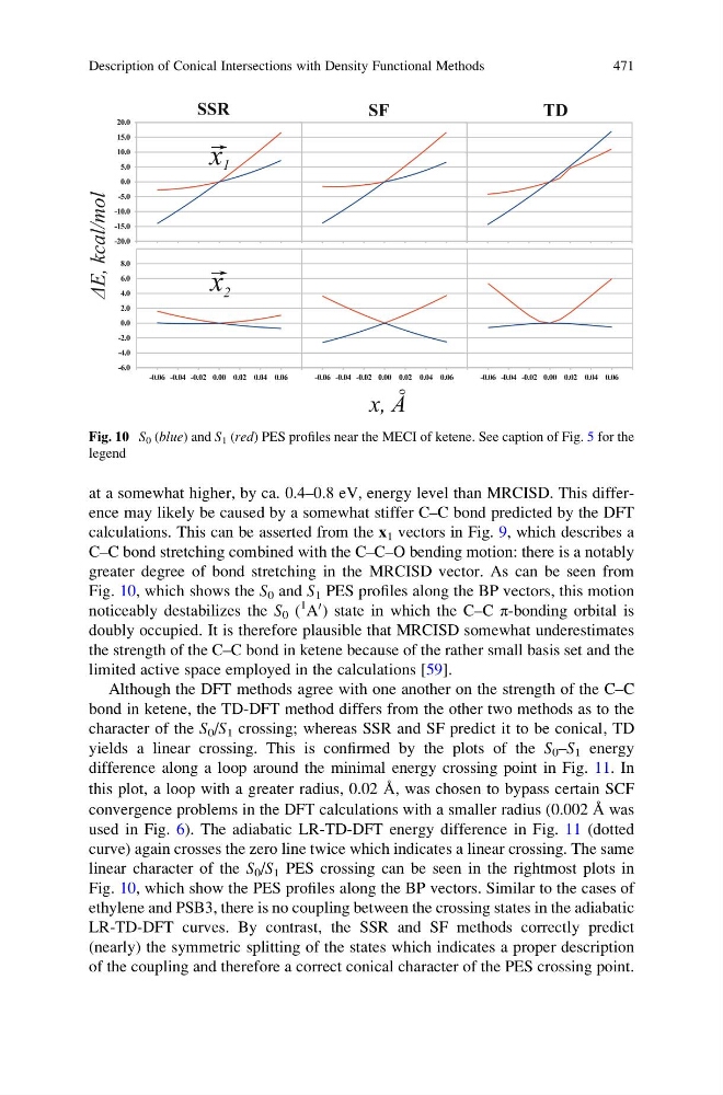
Fig. 10, which shows the S 0 and S 1 PES profiles along the BP vectors, this motion
noticeably destabilizes the S 0 (
1 A
0 ) state in which the C–C π-bonding orbital is
doubly occupied. It is therefore plausible that MRCISD somewhat underestimates
the strength of the C–C bond in ketene because of the rather small basis set and the
limited active space employed in the calculations [59].
Although the DFT methods agree with one another on the strength of the C–C
bond in ketene, the TD-DFT method differs from the other two methods as to the
character of the S 0 /S 1 crossing; whereas SSR and SF predict it to be conical, TD
yields a linear crossing. This is confirmed by the plots of the S 0 –S 1 energy
difference along a loop around the minimal energy crossing point in Fig. 11. In
this plot, a loop with a greater radius, 0.02 Å, was chosen to bypass certain SCF
convergence problems in the DFT calculations with a smaller radius (0.002 Å was
used in Fig. 6). The adiabatic LR-TD-DFT energy difference in Fig. 11 (dotted
curve) again crosses the zero line twice which indicates a linear crossing. The same
linear character of the S 0 /S 1 PES crossing can be seen in the rightmost plots in
Fig. 10, which show the PES profiles along the BP vectors. Similar to the cases of
ethylene and PSB3, there is no coupling between the crossing states in the adiabatic
LR-TD-DFT curves. By contrast, the SSR and SF methods correctly predict
(nearly) the symmetric splitting of the states which indicates a proper description
of the coupling and therefore a correct conical character of the PES crossing point.
Fig. 10 S 0 (blue) and S 1 (red) PES profiles near the MECI of ketene. See caption of Fig. 5 for the
legend
Description of Conical Intersections with Density Functional Methods
471
calculations. This can be asserted from the x 1 vectors in Fig. 9, which describes a
C–C bond stretching combined with the C–C–O bending motion: there is a notably
greater degree of bond stretching in the MRCISD vector. As can be seen from
Fig. 10, which shows the S 0 and S 1 PES profiles along the BP vectors, this motion
noticeably destabilizes the S 0 (
1 A
0 ) state in which the C–C π-bonding orbital is
doubly occupied. It is therefore plausible that MRCISD somewhat underestimates
the strength of the C–C bond in ketene because of the rather small basis set and the
limited active space employed in the calculations [59].
Although the DFT methods agree with one another on the strength of the C–C
bond in ketene, the TD-DFT method differs from the other two methods as to the
character of the S 0 /S 1 crossing; whereas SSR and SF predict it to be conical, TD
yields a linear crossing. This is confirmed by the plots of the S 0 –S 1 energy
difference along a loop around the minimal energy crossing point in Fig. 11. In
this plot, a loop with a greater radius, 0.02 Å, was chosen to bypass certain SCF
convergence problems in the DFT calculations with a smaller radius (0.002 Å was
used in Fig. 6). The adiabatic LR-TD-DFT energy difference in Fig. 11 (dotted
curve) again crosses the zero line twice which indicates a linear crossing. The same
linear character of the S 0 /S 1 PES crossing can be seen in the rightmost plots in
Fig. 10, which show the PES profiles along the BP vectors. Similar to the cases of
ethylene and PSB3, there is no coupling between the crossing states in the adiabatic
LR-TD-DFT curves. By contrast, the SSR and SF methods correctly predict
(nearly) the symmetric splitting of the states which indicates a proper description
of the coupling and therefore a correct conical character of the PES crossing point.
Fig. 10 S 0 (blue) and S 1 (red) PES profiles near the MECI of ketene. See caption of Fig. 5 for the
legend
Description of Conical Intersections with Density Functional Methods
471