

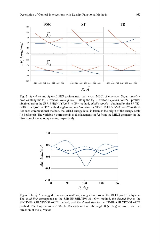
Fig. 5 S 0 (blue) and S 1 (red) PES profiles near the tw-pyr MECI of ethylene. Upper panels –
profiles along the x 1 BP vector, lower panels – along the x 2 BP vector. Leftmost panels – profiles
obtained using the SSR-BH&HLYP/6-31 + G** method, middle panels – obtained by the SF-TDBH&HLYP/6-31 + G** method, rightmost panels – using the TD-BH&HLYP/6-31 + G** method.
For each computational method, the MECI energy level is taken as the origin of the energy scale
(in kcal/mol). The variable x corresponds to displacement (in Å) from the MECI geometry in the
direction of the x 1 or x 2 vector, respectively
Fig. 6 The S 0 –S 1 energy difference (in kcal/mol) along a loop around the MECI point of ethylene.
The solid line corresponds to the SSR-BH&HLYP/6-31 + G** method, the dashed line to the
SF-TD-BH&HLYP/6-31 + G** method, and the dotted line to the TD-BH&HLYP/6-31 + G**
method. The loop radius is 0.002 Å. For each method, the angle θ (in deg) is taken from the
direction of the x 1 vector
Description of Conical Intersections with Density Functional Methods
467
profiles along the x 1 BP vector, lower panels – along the x 2 BP vector. Leftmost panels – profiles
obtained using the SSR-BH&HLYP/6-31 + G** method, middle panels – obtained by the SF-TDBH&HLYP/6-31 + G** method, rightmost panels – using the TD-BH&HLYP/6-31 + G** method.
For each computational method, the MECI energy level is taken as the origin of the energy scale
(in kcal/mol). The variable x corresponds to displacement (in Å) from the MECI geometry in the
direction of the x 1 or x 2 vector, respectively
Fig. 6 The S 0 –S 1 energy difference (in kcal/mol) along a loop around the MECI point of ethylene.
The solid line corresponds to the SSR-BH&HLYP/6-31 + G** method, the dashed line to the
SF-TD-BH&HLYP/6-31 + G** method, and the dotted line to the TD-BH&HLYP/6-31 + G**
method. The loop radius is 0.002 Å. For each method, the angle θ (in deg) is taken from the
direction of the x 1 vector
Description of Conical Intersections with Density Functional Methods
467