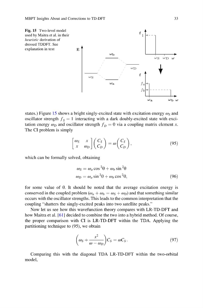
states.) Figure 15 shows a bright singly-excited state with excitation energy ω S and
oscillator strength f S ¼ 1 interacting with a dark doubly-excited state with excitation energy ω D and oscillator strength f D ¼ 0 via a coupling matrix element x.
The CI problem is simply
ω S x
x ω D
!
C S
C D
¼ ω
C S
C D
;
ð95Þ
which can be formally solved, obtaining
ω S ¼ ω a cos
2
θ þ ω b sin
2
θ
ω D ¼ ω a sin
2
θ þ ω b cos
2
θ;
ð96Þ
for some value of θ. It should be noted that the average excitation energy is
conserved in the coupled problem (ω a þ ω b ¼ ω S þ ω D ) and that something similar
occurs with the oscillator strengths. This leads to the common interpretation that the
coupling “shatters the singly-excited peaks into two satellite peaks.”
Now let us see how this wavefunction theory compares with LR-TD-DFT and
how Maitra et al. [61] decided to combine the two into a hybrid method. Of course,
the proper comparison with CI is LR-TD-DFT within the TDA. Applying the
partitioning technique to (95), we obtain
ω S þ
x
2
ω À ω D
C S ¼ ωC S :
ð97Þ
Comparing this with the diagonal TDA LR-TD-DFT within the two-orbital
model,
E
ω S
ω D
ω b
ω a
f
ω
ω S
1
ω D
f
ω
ω a
f a
f b
ω b
Fig. 15 Two-level model
used by Maitra et al. in their
heuristic derivation of
dressed TDDFT. See
explanation in text
MBPT Insights About and Corrections to TD-DFT
33