

Γ ω
ð Þ ¼ ω T
{
T
{
À
Á þ T
{
H
^
T
{
¼
X
I
T
{
T
{
À
Á
Z I ω þ ω I
ð
ÞZ
{
I T
{
T
{
À
Á ; ð85Þ
and
Γ
À1
ω
ð Þ ¼ ω T
{
T
{
À
Á þ T
{
H
^
T
{
h
i À1 ¼
X
I
Z I ω þ ω I
ð
Þ
À1 Z
{
I :
ð86Þ
So (82) reads
ÀΠ sr, q p ω
ð Þ ¼
X
I
^
p
{
^
q
T
{
À
Á
Z I ω þ ω I
ð
Þ
À1 Z
{
I T
{
^
r
{
^
s
À
Á :
ð87Þ
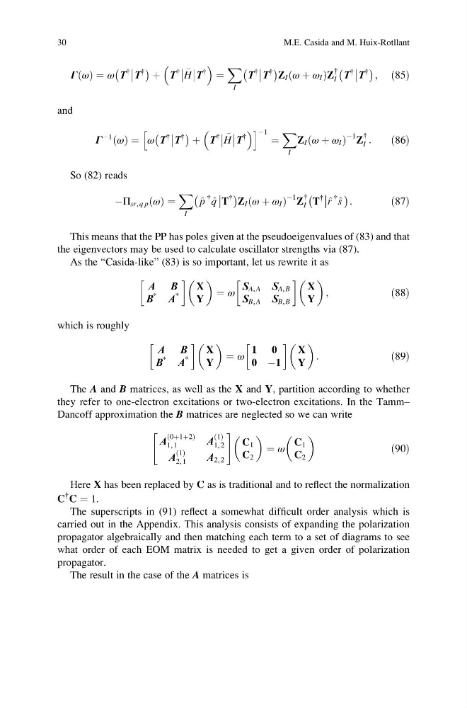
This means that the PP has poles given at the pseudoeigenvalues of (83) and that
the eigenvectors may be used to calculate oscillator strengths via (87).
As the “Casida-like” (83) is so important, let us rewrite it as
A B
B
*
A
*
!
X
Y
¼ ω
S A, A S A, B
S B, A S B, B
!
X
Y
;
ð88Þ
which is roughly
A B
B
*
A
*
!
X
Y
¼ ω
1 0
0 À1
!
X
Y
:
ð89Þ
The A and B matrices, as well as the X and Y, partition according to whether
they refer to one-electron excitations or two-electron excitations. In the Tamm–
Dancoff approximation the B matrices are neglected so we can write
A
0þ1þ2
ð
Þ
1, 1
A
1
ð Þ
1, 2
A
1
ð Þ
2, 1
A 2, 2
"
#
C 1
C 2
¼ ω
C 1
C 2
ð90Þ
Here X has been replaced by C as is traditional and to reflect the normalization
C
{ C ¼ 1.
The superscripts in (91) reflect a somewhat difficult order analysis which is
carried out in the Appendix. This analysis consists of expanding the polarization
propagator algebraically and then matching each term to a set of diagrams to see
what order of each EOM matrix is needed to get a given order of polarization
propagator.
The result in the case of the A matrices is
30
M.E. Casida and M. Huix-Rotllant
ð Þ ¼ ω T
{
T
{
À
Á þ T
{
H
^
T
{
¼
X
I
T
{
T
{
À
Á
Z I ω þ ω I
ð
ÞZ
{
I T
{
T
{
À
Á ; ð85Þ
and
Γ
À1
ω
ð Þ ¼ ω T
{
T
{
À
Á þ T
{
H
^
T
{
h
i À1 ¼
X
I
Z I ω þ ω I
ð
Þ
À1 Z
{
I :
ð86Þ
So (82) reads
ÀΠ sr, q p ω
ð Þ ¼
X
I
^
p
{
^
q
T
{
À
Á
Z I ω þ ω I
ð
Þ
À1 Z
{
I T
{
^
r
{
^
s
À
Á :
ð87Þ
This means that the PP has poles given at the pseudoeigenvalues of (83) and that
the eigenvectors may be used to calculate oscillator strengths via (87).
As the “Casida-like” (83) is so important, let us rewrite it as
A B
B
*
A
*
!
X
Y
¼ ω
S A, A S A, B
S B, A S B, B
!
X
Y
;
ð88Þ
which is roughly
A B
B
*
A
*
!
X
Y
¼ ω
1 0
0 À1
!
X
Y
:
ð89Þ
The A and B matrices, as well as the X and Y, partition according to whether
they refer to one-electron excitations or two-electron excitations. In the Tamm–
Dancoff approximation the B matrices are neglected so we can write
A
0þ1þ2
ð
Þ
1, 1
A
1
ð Þ
1, 2
A
1
ð Þ
2, 1
A 2, 2
"
#
C 1
C 2
¼ ω
C 1
C 2
ð90Þ
Here X has been replaced by C as is traditional and to reflect the normalization
C
{ C ¼ 1.
The superscripts in (91) reflect a somewhat difficult order analysis which is
carried out in the Appendix. This analysis consists of expanding the polarization
propagator algebraically and then matching each term to a set of diagrams to see
what order of each EOM matrix is needed to get a given order of polarization
propagator.
The result in the case of the A matrices is
30
M.E. Casida and M. Huix-Rotllant