

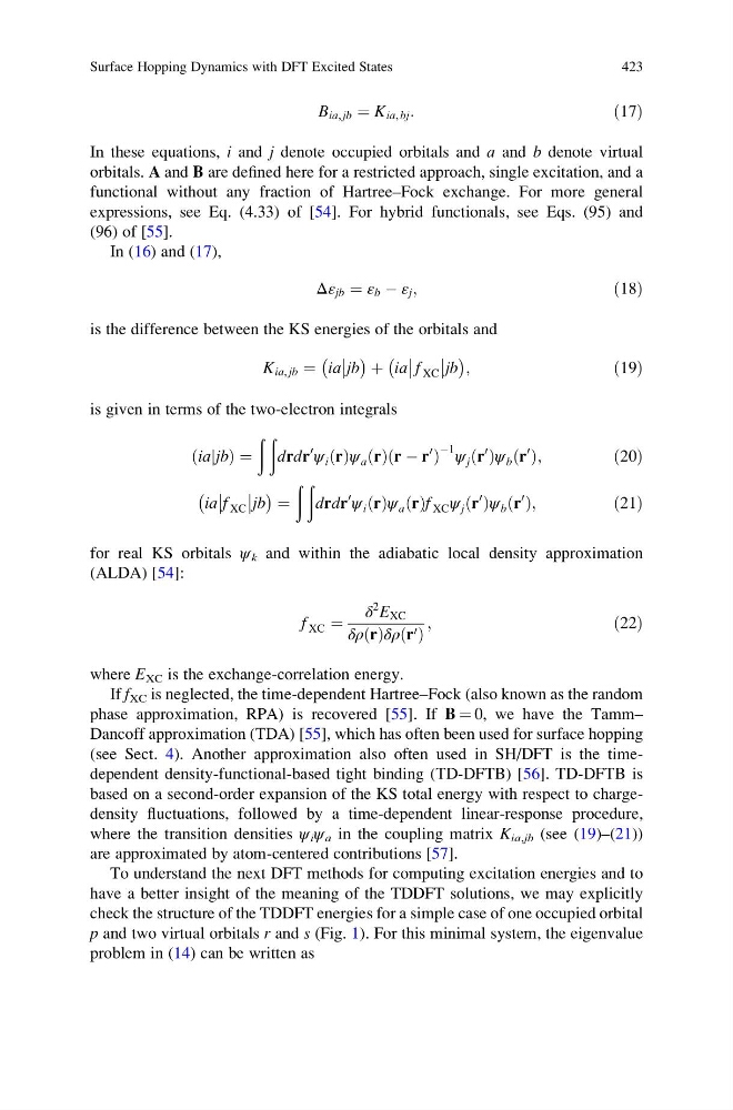
B ia, jb ¼ K ia, bj :
ð17Þ
In these equations, i and j denote occupied orbitals and a and b denote virtual
orbitals. A and B are defined here for a restricted approach, single excitation, and a
functional without any fraction of Hartree–Fock exchange. For more general
expressions, see Eq. (4.33) of [54]. For hybrid functionals, see Eqs. (95) and
(96) of [55].
In (16) and (17),
Δε jb ¼ ε b À ε j ;
ð18Þ
is the difference between the KS energies of the orbitals and
K ia, jb ¼ ia
jb
À
Á þ ia
f XC
jb
À
Á ;
ð19Þ
is given in terms of the two-electron integrals
ia jb
j
ð
Þ¼
ð ð
drdr
0
ψ i r
ð Þψ a r
ð Þ r À r
0
ð
Þ
À1 ψ j r
0
ð Þψ b r
0
ð Þ;
ð20Þ
ia
f XC
jb
À
Á ¼
ð ð
drdr
0
ψ i r
ð Þψ a r
ð Þf XC ψ j r
0
ð Þψ b r
0
ð Þ;
ð21Þ
for real KS orbitals ψ k and within the adiabatic local density approximation
(ALDA) [54]:
f XC ¼
δ
2 E XC
δρ r
ð Þδρ r 0
ð Þ
;
ð22Þ
where E XC is the exchange-correlation energy.
If f XC is neglected, the time-dependent Hartree–Fock (also known as the random
phase approximation, RPA) is recovered [55]. If B ¼ 0, we have the Tamm–
Dancoff approximation (TDA) [55], which has often been used for surface hopping
(see Sect. 4). Another approximation also often used in SH/DFT is the timedependent density-functional-based tight binding (TD-DFTB) [56]. TD-DFTB is
based on a second-order expansion of the KS total energy with respect to chargedensity fluctuations, followed by a time-dependent linear-response procedure,
where the transition densities ψ i ψ a in the coupling matrix K ia,jb (see (19)–(21))
are approximated by atom-centered contributions [57].
To understand the next DFT methods for computing excitation energies and to
have a better insight of the meaning of the TDDFT solutions, we may explicitly
check the structure of the TDDFT energies for a simple case of one occupied orbital
p and two virtual orbitals r and s (Fig. 1). For this minimal system, the eigenvalue
problem in (14) can be written as
Surface Hopping Dynamics with DFT Excited States
423
ð17Þ
In these equations, i and j denote occupied orbitals and a and b denote virtual
orbitals. A and B are defined here for a restricted approach, single excitation, and a
functional without any fraction of Hartree–Fock exchange. For more general
expressions, see Eq. (4.33) of [54]. For hybrid functionals, see Eqs. (95) and
(96) of [55].
In (16) and (17),
Δε jb ¼ ε b À ε j ;
ð18Þ
is the difference between the KS energies of the orbitals and
K ia, jb ¼ ia
jb
À
Á þ ia
f XC
jb
À
Á ;
ð19Þ
is given in terms of the two-electron integrals
ia jb
j
ð
Þ¼
ð ð
drdr
0
ψ i r
ð Þψ a r
ð Þ r À r
0
ð
Þ
À1 ψ j r
0
ð Þψ b r
0
ð Þ;
ð20Þ
ia
f XC
jb
À
Á ¼
ð ð
drdr
0
ψ i r
ð Þψ a r
ð Þf XC ψ j r
0
ð Þψ b r
0
ð Þ;
ð21Þ
for real KS orbitals ψ k and within the adiabatic local density approximation
(ALDA) [54]:
f XC ¼
δ
2 E XC
δρ r
ð Þδρ r 0
ð Þ
;
ð22Þ
where E XC is the exchange-correlation energy.
If f XC is neglected, the time-dependent Hartree–Fock (also known as the random
phase approximation, RPA) is recovered [55]. If B ¼ 0, we have the Tamm–
Dancoff approximation (TDA) [55], which has often been used for surface hopping
(see Sect. 4). Another approximation also often used in SH/DFT is the timedependent density-functional-based tight binding (TD-DFTB) [56]. TD-DFTB is
based on a second-order expansion of the KS total energy with respect to chargedensity fluctuations, followed by a time-dependent linear-response procedure,
where the transition densities ψ i ψ a in the coupling matrix K ia,jb (see (19)–(21))
are approximated by atom-centered contributions [57].
To understand the next DFT methods for computing excitation energies and to
have a better insight of the meaning of the TDDFT solutions, we may explicitly
check the structure of the TDDFT energies for a simple case of one occupied orbital
p and two virtual orbitals r and s (Fig. 1). For this minimal system, the eigenvalue
problem in (14) can be written as
Surface Hopping Dynamics with DFT Excited States
423