

Surface hopping is not restricted to internal conversion, and other types of
nonadiabatic transitions may be considered, such as those induced by spin-orbit
couplings (intersystem crossing) [45, 46] or electromagnetic fields [47–50]. From a
general standpoint, to consider these effects it is sufficient to redefine the coupling
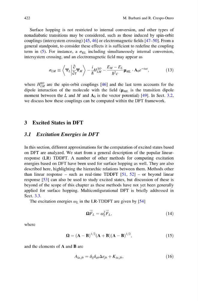
term in (5). For instance, a σ KL including simultaneously internal conversion,
intersystem crossing, and an electromagnetic field may appear as
σ LM Ψ L
∂
∂t
Ψ M
(
)
À
i
h
H
SO
LM À
E M À E L
h
2 c
μ ML Á A 0 e
Àiωt
;
ð13Þ
where H
SO
LM are the spin-orbit couplings [46] and the last term accounts for the
dipole interaction of the molecule with the field (μ ML is the transition dipole
moment between the L and M and A 0 is the vector potential) [49]. In Sect. 3.2,
we discuss how these couplings can be computed within the DFT framework.
3 Excited States in DFT
3.1 Excitation Energies in DFT
In this section, different approximations for the computation of excited states based
on DFT are analyzed. We start from a general description of the popular linearresponse (LR) TDDFT. A number of other methods for computing excitation
energies based on DFT have been used for surface hopping as well. They are also
described here, highlighting the hierarchic relations between them. Methods other
than linear response – such as real-time TDDFT [51, 52] – or beyond linear
response [53] can also be used to study excited states, but discussion of these is
beyond of the scope of this chapter as these methods have not yet been generally
applied for surface hopping. Multiconfigurational DFT is briefly addressed in
Sect. 3.3.
The excitation energies ω L in the LR-TDDFT are given by [54]
ΩF
!
L ¼ ω
2
L F
!
L ;
ð14Þ
where
Ω ¼ A À B
ð
Þ
1=2 A þ B
ð
Þ A À B
ð
Þ
1=2 ;
ð15Þ
and the elements of A and B are
A ia, jb ¼ δ ij δ ab Δε jb þ K ia, jb ;
ð16Þ
422
M. Barbatti and R. Crespo-Otero
nonadiabatic transitions may be considered, such as those induced by spin-orbit
couplings (intersystem crossing) [45, 46] or electromagnetic fields [47–50]. From a
general standpoint, to consider these effects it is sufficient to redefine the coupling
term in (5). For instance, a σ KL including simultaneously internal conversion,
intersystem crossing, and an electromagnetic field may appear as
σ LM Ψ L
∂
∂t
Ψ M
(
)
À
i
h
H
SO
LM À
E M À E L
h
2 c
μ ML Á A 0 e
Àiωt
;
ð13Þ
where H
SO
LM are the spin-orbit couplings [46] and the last term accounts for the
dipole interaction of the molecule with the field (μ ML is the transition dipole
moment between the L and M and A 0 is the vector potential) [49]. In Sect. 3.2,
we discuss how these couplings can be computed within the DFT framework.
3 Excited States in DFT
3.1 Excitation Energies in DFT
In this section, different approximations for the computation of excited states based
on DFT are analyzed. We start from a general description of the popular linearresponse (LR) TDDFT. A number of other methods for computing excitation
energies based on DFT have been used for surface hopping as well. They are also
described here, highlighting the hierarchic relations between them. Methods other
than linear response – such as real-time TDDFT [51, 52] – or beyond linear
response [53] can also be used to study excited states, but discussion of these is
beyond of the scope of this chapter as these methods have not yet been generally
applied for surface hopping. Multiconfigurational DFT is briefly addressed in
Sect. 3.3.
The excitation energies ω L in the LR-TDDFT are given by [54]
ΩF
!
L ¼ ω
2
L F
!
L ;
ð14Þ
where
Ω ¼ A À B
ð
Þ
1=2 A þ B
ð
Þ A À B
ð
Þ
1=2 ;
ð15Þ
and the elements of A and B are
A ia, jb ¼ δ ij δ ab Δε jb þ K ia, jb ;
ð16Þ
422
M. Barbatti and R. Crespo-Otero