

Π
diag
sr, q p ω
ð Þ ¼
X
a, b, c, i, k, l
pq
ba
À
Á
kl
rs
À
Á
ε ik, bc ω À ε ik, ca
ð
Þ ε il, ac
;
ð68Þ
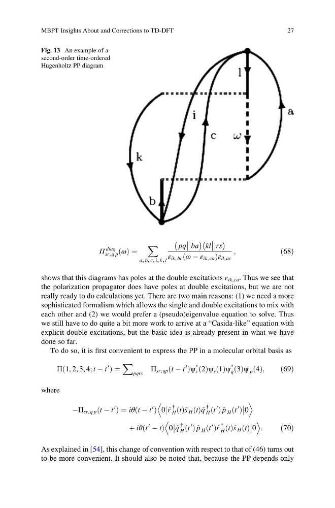
shows that this diagrams has poles at the double excitations ε ik,ca . Thus we see that
the polarization propagator does have poles at double excitations, but we are not
really ready to do calculations yet. There are two main reasons: (1) we need a more
sophisticated formalism which allows the single and double excitations to mix with
each other and (2) we would prefer a (pseudo)eigenvalue equation to solve. Thus
we still have to do quite a bit more work to arrive at a “Casida-like” equation with
explicit double excitations, but the basic idea is already present in what we have
done so far.
To do so, it is first convenient to express the PP in a molecular orbital basis as
Π 1, 2, 3, 4; t À t
0
ð
Þ ¼
X
pqrs
Π sr, qp t À t
0
ð
Þψ
*
r 2
ð Þψ s 1
ð Þψ
*
q 3
ð Þψ p 4
ð Þ;
ð69Þ
where
ÀΠ sr, q p t À t
0
ð
Þ¼iθ t À t
0
ð
Þ 0
^
r
{
H t
ð Þ^ s H t
ð Þ^ q
{
H t
0
ð Þ^ p H t
0
ð Þ
0
D
E
þ iθ t
0
À t
ð
Þ 0
^
q
{
H t
0
ð Þ^ p H t
0
ð Þ^ r
{
H t
ð Þ^ s H t
ð Þ
0
D
E
:
ð70Þ
As explained in [54], this change of convention with respect to that of (46) turns out
to be more convenient. It should also be noted that, because the PP depends only
Fig. 13 An example of a
second-order time-ordered
Hugenholtz PP diagram
MBPT Insights About and Corrections to TD-DFT
27
diag
sr, q p ω
ð Þ ¼
X
a, b, c, i, k, l
pq
ba
À
Á
kl
rs
À
Á
ε ik, bc ω À ε ik, ca
ð
Þ ε il, ac
;
ð68Þ
shows that this diagrams has poles at the double excitations ε ik,ca . Thus we see that
the polarization propagator does have poles at double excitations, but we are not
really ready to do calculations yet. There are two main reasons: (1) we need a more
sophisticated formalism which allows the single and double excitations to mix with
each other and (2) we would prefer a (pseudo)eigenvalue equation to solve. Thus
we still have to do quite a bit more work to arrive at a “Casida-like” equation with
explicit double excitations, but the basic idea is already present in what we have
done so far.
To do so, it is first convenient to express the PP in a molecular orbital basis as
Π 1, 2, 3, 4; t À t
0
ð
Þ ¼
X
pqrs
Π sr, qp t À t
0
ð
Þψ
*
r 2
ð Þψ s 1
ð Þψ
*
q 3
ð Þψ p 4
ð Þ;
ð69Þ
where
ÀΠ sr, q p t À t
0
ð
Þ¼iθ t À t
0
ð
Þ 0
^
r
{
H t
ð Þ^ s H t
ð Þ^ q
{
H t
0
ð Þ^ p H t
0
ð Þ
0
D
E
þ iθ t
0
À t
ð
Þ 0
^
q
{
H t
0
ð Þ^ p H t
0
ð Þ^ r
{
H t
ð Þ^ s H t
ð Þ
0
D
E
:
ð70Þ
As explained in [54], this change of convention with respect to that of (46) turns out
to be more convenient. It should also be noted that, because the PP depends only
Fig. 13 An example of a
second-order time-ordered
Hugenholtz PP diagram
MBPT Insights About and Corrections to TD-DFT
27