

Defining order as the order in the number of times ^
V and/or ^
M xc appear, all of the
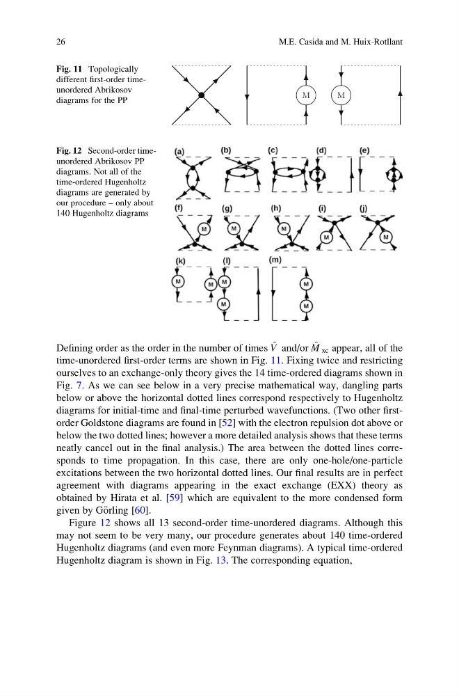
time-unordered first-order terms are shown in Fig. 11. Fixing twice and restricting
ourselves to an exchange-only theory gives the 14 time-ordered diagrams shown in
Fig. 7. As we can see below in a very precise mathematical way, dangling parts
below or above the horizontal dotted lines correspond respectively to Hugenholtz
diagrams for initial-time and final-time perturbed wavefunctions. (Two other firstorder Goldstone diagrams are found in [52] with the electron repulsion dot above or
below the two dotted lines; however a more detailed analysis shows that these terms
neatly cancel out in the final analysis.) The area between the dotted lines corresponds to time propagation. In this case, there are only one-hole/one-particle
excitations between the two horizontal dotted lines. Our final results are in perfect
agreement with diagrams appearing in the exact exchange (EXX) theory as
obtained by Hirata et al. [59] which are equivalent to the more condensed form
given by G€ orling [60].
Figure 12 shows all 13 second-order time-unordered diagrams. Although this
may not seem to be very many, our procedure generates about 140 time-ordered
Hugenholtz diagrams (and even more Feynman diagrams). A typical time-ordered
Hugenholtz diagram is shown in Fig. 13. The corresponding equation,
M
M
Fig. 11 Topologically
different first-order timeunordered Abrikosov
diagrams for the PP
Fig. 12 Second-order timeunordered Abrikosov PP
diagrams. Not all of the
time-ordered Hugenholtz
diagrams are generated by
our procedure – only about
140 Hugenholtz diagrams
26
M.E. Casida and M. Huix-Rotllant
V and/or ^
M xc appear, all of the
time-unordered first-order terms are shown in Fig. 11. Fixing twice and restricting
ourselves to an exchange-only theory gives the 14 time-ordered diagrams shown in
Fig. 7. As we can see below in a very precise mathematical way, dangling parts
below or above the horizontal dotted lines correspond respectively to Hugenholtz
diagrams for initial-time and final-time perturbed wavefunctions. (Two other firstorder Goldstone diagrams are found in [52] with the electron repulsion dot above or
below the two dotted lines; however a more detailed analysis shows that these terms
neatly cancel out in the final analysis.) The area between the dotted lines corresponds to time propagation. In this case, there are only one-hole/one-particle
excitations between the two horizontal dotted lines. Our final results are in perfect
agreement with diagrams appearing in the exact exchange (EXX) theory as
obtained by Hirata et al. [59] which are equivalent to the more condensed form
given by G€ orling [60].
Figure 12 shows all 13 second-order time-unordered diagrams. Although this
may not seem to be very many, our procedure generates about 140 time-ordered
Hugenholtz diagrams (and even more Feynman diagrams). A typical time-ordered
Hugenholtz diagram is shown in Fig. 13. The corresponding equation,
M
M
Fig. 11 Topologically
different first-order timeunordered Abrikosov
diagrams for the PP
Fig. 12 Second-order timeunordered Abrikosov PP
diagrams. Not all of the
time-ordered Hugenholtz
diagrams are generated by
our procedure – only about
140 Hugenholtz diagrams
26
M.E. Casida and M. Huix-Rotllant