

10. An additional factor of 1/2 must be added for each pair of equivalent lines.
These are directed lines whose interchange, in the absence of further labeling,
leaves the Hugenholtz diagram unchanged.
For example, the term corresponding to Fig. 7a is
Π ck, ai ω
ð Þ ¼ À
ka
ic
À
Á
Àω þ ε k À ε c
ð
ÞÀ ω þ ε i À ε a
ð
Þ
¼
ak
ic
À
Á
Àω þ ε k À ε c
ð
ÞÀ ω þ ε i À ε a
ð
Þ
:
ð58Þ
Additional information about Hugenholtz and other diagrams may be found,
for example, in [56].
3.3 Dyson’s Equation and the Bethe–Salpeter Equation
(BSE)
Two of the most basic equations of diagrammatic MBPT are Dyson’s equation for
the one-electron Green’s function and the BSE for the ph-propagator. Both require
the choice of a zero-order picture which we take here to be the exact or approximate
Kohn–Sham system of noninteracting electrons. We denote the zero-order quantities by the subscript s (for single particle).
Dyson’s equation relates the true one-electron Green’s function G to the zeroorder Green’s function G s via the (proper) self-energy Σ,
G 1; 2
ð Þ ¼ G s 1; 2
ð Þþ
ð
G s 1; 3
ð ÞΣ 3; 4
ð ÞG 4; 2
ð Þd3d4;
ð59Þ
or, more concisely,
G ¼ G s þ G s ΣG :
ð60Þ
This is shown diagrammatically in Fig. 9. It is to be emphasized that these
diagrams are unordered in time as it is not possible to write a Dyson equation for
time-ordered diagrams. Also shown in Fig. 9 are typical low-order self-energy
approximations. Typical quantum chemistry approximations (Fig. 9b) involve
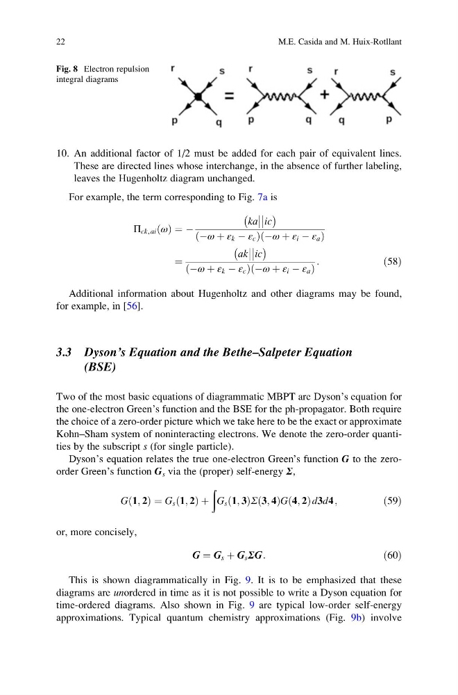
Fig. 8 Electron repulsion
integral diagrams
22
M.E. Casida and M. Huix-Rotllant
These are directed lines whose interchange, in the absence of further labeling,
leaves the Hugenholtz diagram unchanged.
For example, the term corresponding to Fig. 7a is
Π ck, ai ω
ð Þ ¼ À
ka
ic
À
Á
Àω þ ε k À ε c
ð
ÞÀ ω þ ε i À ε a
ð
Þ
¼
ak
ic
À
Á
Àω þ ε k À ε c
ð
ÞÀ ω þ ε i À ε a
ð
Þ
:
ð58Þ
Additional information about Hugenholtz and other diagrams may be found,
for example, in [56].
3.3 Dyson’s Equation and the Bethe–Salpeter Equation
(BSE)
Two of the most basic equations of diagrammatic MBPT are Dyson’s equation for
the one-electron Green’s function and the BSE for the ph-propagator. Both require
the choice of a zero-order picture which we take here to be the exact or approximate
Kohn–Sham system of noninteracting electrons. We denote the zero-order quantities by the subscript s (for single particle).
Dyson’s equation relates the true one-electron Green’s function G to the zeroorder Green’s function G s via the (proper) self-energy Σ,
G 1; 2
ð Þ ¼ G s 1; 2
ð Þþ
ð
G s 1; 3
ð ÞΣ 3; 4
ð ÞG 4; 2
ð Þd3d4;
ð59Þ
or, more concisely,
G ¼ G s þ G s ΣG :
ð60Þ
This is shown diagrammatically in Fig. 9. It is to be emphasized that these
diagrams are unordered in time as it is not possible to write a Dyson equation for
time-ordered diagrams. Also shown in Fig. 9 are typical low-order self-energy
approximations. Typical quantum chemistry approximations (Fig. 9b) involve
Fig. 8 Electron repulsion
integral diagrams
22
M.E. Casida and M. Huix-Rotllant