

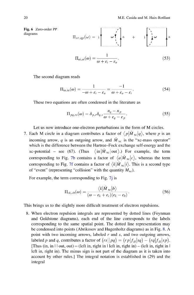
Π ai, ai ω
ð Þ ¼
1
ω þ ε i À ε a
:
ð53Þ
The second diagram reads
Π ia, ia ω
ð Þ ¼
1
Àω þ ε i À ε a
¼
À1
ω þ ε a À ε i
:
ð54Þ
These two equations are often condensed in the literature as
Π pq, rs ω
ð Þ ¼ δ p, r δ q, s
n q À n p
ω þ ε q À ε p
:
ð55Þ
Let us now introduce one-electron perturbations in the form of M circles.
7. Each M circle in a diagram contributes a factor of p
^
M xc
q
, where p is an
incoming arrow, q is an outgoing arrow, and ^
M xc is the “xc-mass operator”
which is the difference between the Hartree–Fock exchange self-energy and the
xc-potential – see (67). (Thus
in
^
M xc
out
.) For example, the term
corresponding to Fig. 7b contains a factor of a
^
M xc
c
, whereas the term
corresponding to Fig. 7f contains a factor of k
^
M xc
i
. This is a second type
of “event” (representing “collision” with the quantity M xc ).
For example, the term corresponding to Fig. 7j is
Π ck, cb ω
ð Þ ¼
k
^
M xc
b
ω À ε k þ ε c
ð
Þε k À ε b
ð
Þ
:
ð56Þ
This brings us to the slightly more difficult treatment of electron repulsions.
8. When electron repulsion integrals are represented by dotted lines (Feynman
and Goldstone diagrams), each end of the line corresponds to the labels
corresponding to the same spatial point. The dotted line representation may
be condensed into points (Abrikosov and Hugenholtz diagrams) as in Fig. 8. A
point with two incoming arrows, labeled r and s, and two outgoing arrows,
labeled p and q, contributes a factor of rs
pq
À
Á ¼ r p
f H
sq
À
Á À rq
f H
s p
À
Á
.
[Thus (in, in | | out, out) ¼ (left in, right in | left in, right in) – (left in, right in |
left in, right in). The minus sign is not part of the diagram as it is taken into
account by other rules.] The integral notation is established in (29) and the
integral
Π sr,qp ( ) =
+
i
a
ω
i
a
ω
ω
Fig. 6 Zero-order PP
diagrams
20
M.E. Casida and M. Huix-Rotllant
ð Þ ¼
1
ω þ ε i À ε a
:
ð53Þ
The second diagram reads
Π ia, ia ω
ð Þ ¼
1
Àω þ ε i À ε a
¼
À1
ω þ ε a À ε i
:
ð54Þ
These two equations are often condensed in the literature as
Π pq, rs ω
ð Þ ¼ δ p, r δ q, s
n q À n p
ω þ ε q À ε p
:
ð55Þ
Let us now introduce one-electron perturbations in the form of M circles.
7. Each M circle in a diagram contributes a factor of p
^
M xc
q
, where p is an
incoming arrow, q is an outgoing arrow, and ^
M xc is the “xc-mass operator”
which is the difference between the Hartree–Fock exchange self-energy and the
xc-potential – see (67). (Thus
in
^
M xc
out
.) For example, the term
corresponding to Fig. 7b contains a factor of a
^
M xc
c
, whereas the term
corresponding to Fig. 7f contains a factor of k
^
M xc
i
. This is a second type
of “event” (representing “collision” with the quantity M xc ).
For example, the term corresponding to Fig. 7j is
Π ck, cb ω
ð Þ ¼
k
^
M xc
b
ω À ε k þ ε c
ð
Þε k À ε b
ð
Þ
:
ð56Þ
This brings us to the slightly more difficult treatment of electron repulsions.
8. When electron repulsion integrals are represented by dotted lines (Feynman
and Goldstone diagrams), each end of the line corresponds to the labels
corresponding to the same spatial point. The dotted line representation may
be condensed into points (Abrikosov and Hugenholtz diagrams) as in Fig. 8. A
point with two incoming arrows, labeled r and s, and two outgoing arrows,
labeled p and q, contributes a factor of rs
pq
À
Á ¼ r p
f H
sq
À
Á À rq
f H
s p
À
Á
.
[Thus (in, in | | out, out) ¼ (left in, right in | left in, right in) – (left in, right in |
left in, right in). The minus sign is not part of the diagram as it is taken into
account by other rules.] The integral notation is established in (29) and the
integral
Π sr,qp ( ) =
+
i
a
ω
i
a
ω
ω
Fig. 6 Zero-order PP
diagrams
20
M.E. Casida and M. Huix-Rotllant