

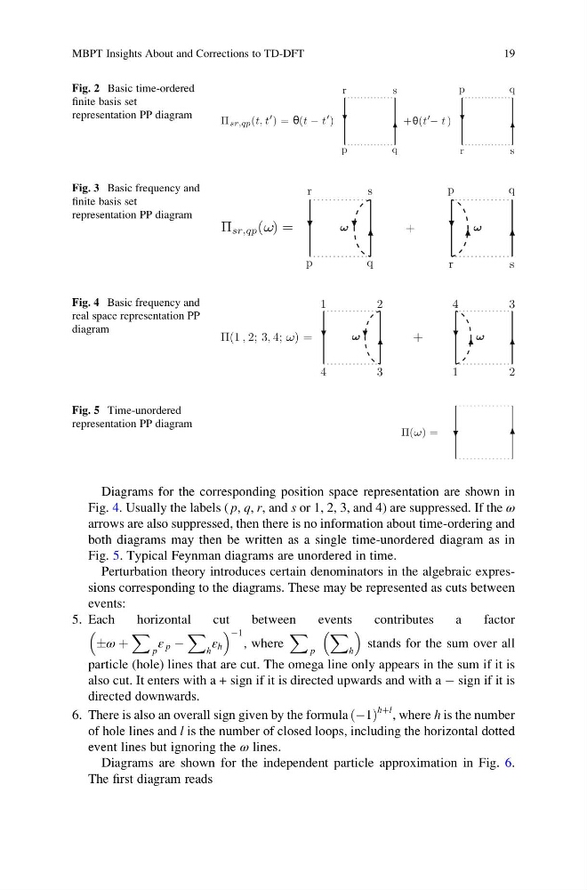
Diagrams for the corresponding position space representation are shown in
Fig. 4. Usually the labels ( p, q, r, and s or 1, 2, 3, and 4) are suppressed. If the ω
arrows are also suppressed, then there is no information about time-ordering and
both diagrams may then be written as a single time-unordered diagram as in
Fig. 5. Typical Feynman diagrams are unordered in time.
Perturbation theory introduces certain denominators in the algebraic expressions corresponding to the diagrams. These may be represented as cuts between
events:
5. Each
horizontal
cut
between
events
contributes
a
factor
Æω þ
X
p
ε p À
X
h
ε h
À1
, where
X
p
X
h
stands for the sum over all
particle (hole) lines that are cut. The omega line only appears in the sum if it is
also cut. It enters with a + sign if it is directed upwards and with a À sign if it is
directed downwards.
6. There is also an overall sign given by the formula À1
ð Þ
hþl , where h is the number
of hole lines and l is the number of closed loops, including the horizontal dotted
event lines but ignoring the ω lines.
Diagrams are shown for the independent particle approximation in Fig. 6.
The first diagram reads
Π sr,qp (t; t
) = θ(t − t
)
+θ(t − t
)
r
s
p
q
r
s
p
q
Fig. 2 Basic time-ordered
finite basis set
representation PP diagram
Π sr,qp (ω) =
+
r
s
p
q
ω
r
s
p
q
ω
Fig. 3 Basic frequency and
finite basis set
representation PP diagram
Π(1 ; 2; 3; 4; ) =
+
1
2
4
3
ω
1
2
4
3
ω
ω
Fig. 4 Basic frequency and
real space representation PP
diagram
Π(ω) =
Fig. 5 Time-unordered
representation PP diagram
MBPT Insights About and Corrections to TD-DFT
19
Fig. 4. Usually the labels ( p, q, r, and s or 1, 2, 3, and 4) are suppressed. If the ω
arrows are also suppressed, then there is no information about time-ordering and
both diagrams may then be written as a single time-unordered diagram as in
Fig. 5. Typical Feynman diagrams are unordered in time.
Perturbation theory introduces certain denominators in the algebraic expressions corresponding to the diagrams. These may be represented as cuts between
events:
5. Each
horizontal
cut
between
events
contributes
a
factor
Æω þ
X
p
ε p À
X
h
ε h
À1
, where
X
p
X
h
stands for the sum over all
particle (hole) lines that are cut. The omega line only appears in the sum if it is
also cut. It enters with a + sign if it is directed upwards and with a À sign if it is
directed downwards.
6. There is also an overall sign given by the formula À1
ð Þ
hþl , where h is the number
of hole lines and l is the number of closed loops, including the horizontal dotted
event lines but ignoring the ω lines.
Diagrams are shown for the independent particle approximation in Fig. 6.
The first diagram reads
Π sr,qp (t; t
) = θ(t − t
)
+θ(t − t
)
r
s
p
q
r
s
p
q
Fig. 2 Basic time-ordered
finite basis set
representation PP diagram
Π sr,qp (ω) =
+
r
s
p
q
ω
r
s
p
q
ω
Fig. 3 Basic frequency and
finite basis set
representation PP diagram
Π(1 ; 2; 3; 4; ) =
+
1
2
4
3
ω
1
2
4
3
ω
ω
Fig. 4 Basic frequency and
real space representation PP
diagram
Π(ω) =
Fig. 5 Time-unordered
representation PP diagram
MBPT Insights About and Corrections to TD-DFT
19