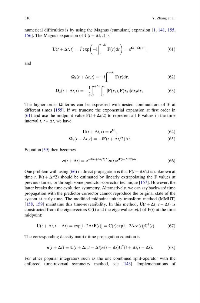
numerical difficulties is by using the Magnus (cumulant) expansion [1, 141, 155,
156]. The Magnus expansion of U(t þ Δt, t) is
U t þ Δt, t
ð
Þ¼ ^
T exp Ài
ð tþΔt
t
F τ
ð Þdτ
¼ e
Ω 1 þΩ 2 þÁÁÁ
;
ð61Þ
and
Ω 1 t þ Δt, t
ð
Þ¼À i
ð tþΔt
t
F τ
ð Þdτ;
ð62Þ
Ω 2 t þ Δt, t
ð
޼1
2
ð tþΔt
t
ð τ 1
t
F τ 1
ð Þ, F τ 2
ð Þ
½
Š dτ 2 dτ 1 :
ð63Þ
The higher order Ω terms can be expressed with nested commutators of F at
different times [155]. If we truncate the exponential expansion at first order in
(61) and use the midpoint value F(t þ Δt/2) to represent all F values in the time
interval t, t + Δt, we have
U t þ Δt, t
ð
Þ¼e
Ω 1 ;
ð64Þ
Ω 1 t þ Δt, t
ð
Þ¼À iF t þ Δt=2
ð
Þ Δt:
ð65Þ
Equation (59) then becomes
σ t þ Δt
ð
Þ¼e
ÀiF tþΔt=2
ð
Þ Δt
σ t
ð Þe
iF tþΔt=2
ð
Þ Δt
:
ð66Þ
One problem with using (66) in direct propagation is that F(t þ Δt/2) is unknown at
time t. F(t þ Δt/2) should be estimated by linearly extrapolating the F values at
previous times, or through some predictor-corrector technique [157]. However, the
latter breaks the time evolution symmetry. Alternatively, we can say backward time
propagation with the predictor-corrector cannot reproduce the original state of the
system at early time. The modified midpoint unitary transform method (MMUT)
[158, 159] maintains this time-reversibility. In this method, U(t þ Δt, t À Δt) is
constructed from the eigenvectors C(t) and the eigenvalues ε(t) of F(t) at the time
midpoint:
U t þ Δt, t À Δt
ð
Þ¼exp i Á 2Δt F t
ð Þ
½
Š¼C t
ð Þexp i Á 2Δt ε t
ð Þ
½
Š C
{ t
ð Þ:
ð67Þ
The corresponding density matrix time propagation equation is
σ t þ Δt
ð
Þ¼U t þ Δt, t À Δt
ð
Þ σ t À Δt
ð
ÞU
{ t þ Δt, t À Δt
ð
Þ :
ð68Þ
For other popular integrators such as the one combined split-operator with the
enforced time-reversal symmetry method, see [143]. Implementations of
310
Y. Zhang et al.