

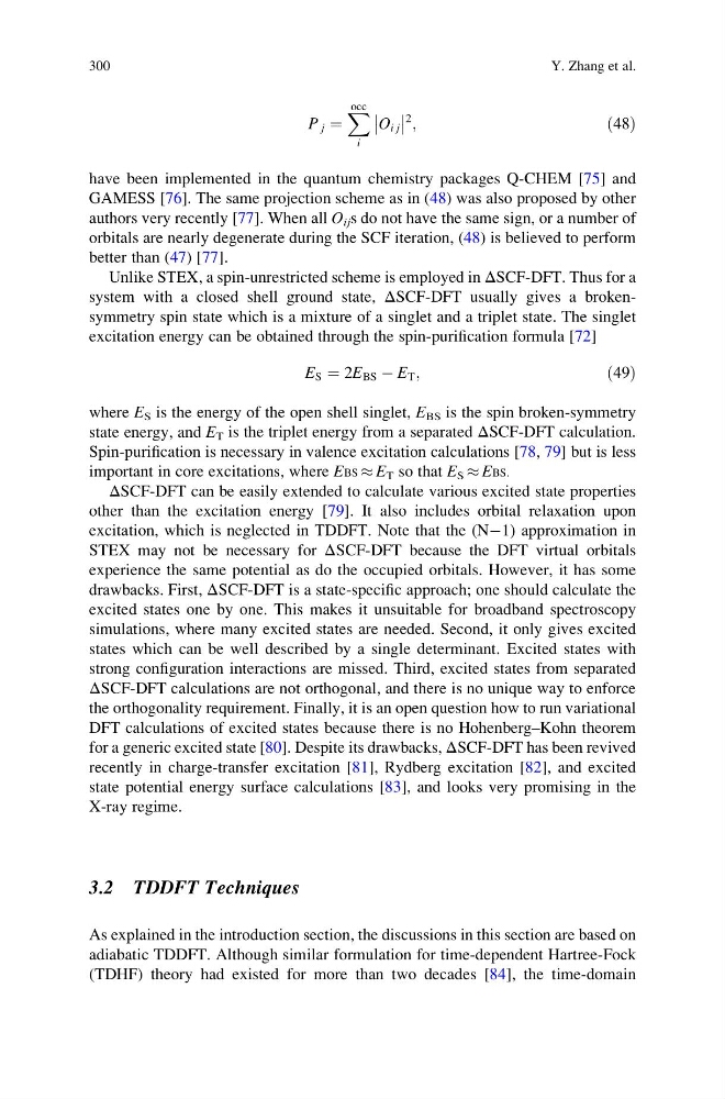
P j ¼
X occ
i
O i j
2 ;
ð48Þ
have been implemented in the quantum chemistry packages Q-CHEM [75] and
GAMESS [76]. The same projection scheme as in (48) was also proposed by other
authors very recently [77]. When all O ij s do not have the same sign, or a number of
orbitals are nearly degenerate during the SCF iteration, (48) is believed to perform
better than (47) [77].
Unlike STEX, a spin-unrestricted scheme is employed in ΔSCF-DFT. Thus for a
system with a closed shell ground state, ΔSCF-DFT usually gives a brokensymmetry spin state which is a mixture of a singlet and a triplet state. The singlet
excitation energy can be obtained through the spin-purification formula [72]
E S ¼ 2E BS À E T ;
ð49Þ
where E S is the energy of the open shell singlet, E BS is the spin broken-symmetry
state energy, and E T is the triplet energy from a separated ΔSCF-DFT calculation.
Spin-purification is necessary in valence excitation calculations [78, 79] but is less
important in core excitations, where EBS % E T so that E S % EBS.
ΔSCF-DFT can be easily extended to calculate various excited state properties
other than the excitation energy [79]. It also includes orbital relaxation upon
excitation, which is neglected in TDDFT. Note that the (NÀ1) approximation in
STEX may not be necessary for ΔSCF-DFT because the DFT virtual orbitals
experience the same potential as do the occupied orbitals. However, it has some
drawbacks. First, ΔSCF-DFT is a state-specific approach; one should calculate the
excited states one by one. This makes it unsuitable for broadband spectroscopy
simulations, where many excited states are needed. Second, it only gives excited
states which can be well described by a single determinant. Excited states with
strong configuration interactions are missed. Third, excited states from separated
ΔSCF-DFT calculations are not orthogonal, and there is no unique way to enforce
the orthogonality requirement. Finally, it is an open question how to run variational
DFT calculations of excited states because there is no Hohenberg–Kohn theorem
for a generic excited state [80]. Despite its drawbacks, ΔSCF-DFT has been revived
recently in charge-transfer excitation [81], Rydberg excitation [82], and excited
state potential energy surface calculations [83], and looks very promising in the
X-ray regime.
3.2 TDDFT Techniques
As explained in the introduction section, the discussions in this section are based on
adiabatic TDDFT. Although similar formulation for time-dependent Hartree-Fock
(TDHF) theory had existed for more than two decades [84], the time-domain
300
Y. Zhang et al.
X occ
i
O i j
2 ;
ð48Þ
have been implemented in the quantum chemistry packages Q-CHEM [75] and
GAMESS [76]. The same projection scheme as in (48) was also proposed by other
authors very recently [77]. When all O ij s do not have the same sign, or a number of
orbitals are nearly degenerate during the SCF iteration, (48) is believed to perform
better than (47) [77].
Unlike STEX, a spin-unrestricted scheme is employed in ΔSCF-DFT. Thus for a
system with a closed shell ground state, ΔSCF-DFT usually gives a brokensymmetry spin state which is a mixture of a singlet and a triplet state. The singlet
excitation energy can be obtained through the spin-purification formula [72]
E S ¼ 2E BS À E T ;
ð49Þ
where E S is the energy of the open shell singlet, E BS is the spin broken-symmetry
state energy, and E T is the triplet energy from a separated ΔSCF-DFT calculation.
Spin-purification is necessary in valence excitation calculations [78, 79] but is less
important in core excitations, where EBS % E T so that E S % EBS.
ΔSCF-DFT can be easily extended to calculate various excited state properties
other than the excitation energy [79]. It also includes orbital relaxation upon
excitation, which is neglected in TDDFT. Note that the (NÀ1) approximation in
STEX may not be necessary for ΔSCF-DFT because the DFT virtual orbitals
experience the same potential as do the occupied orbitals. However, it has some
drawbacks. First, ΔSCF-DFT is a state-specific approach; one should calculate the
excited states one by one. This makes it unsuitable for broadband spectroscopy
simulations, where many excited states are needed. Second, it only gives excited
states which can be well described by a single determinant. Excited states with
strong configuration interactions are missed. Third, excited states from separated
ΔSCF-DFT calculations are not orthogonal, and there is no unique way to enforce
the orthogonality requirement. Finally, it is an open question how to run variational
DFT calculations of excited states because there is no Hohenberg–Kohn theorem
for a generic excited state [80]. Despite its drawbacks, ΔSCF-DFT has been revived
recently in charge-transfer excitation [81], Rydberg excitation [82], and excited
state potential energy surface calculations [83], and looks very promising in the
X-ray regime.
3.2 TDDFT Techniques
As explained in the introduction section, the discussions in this section are based on
adiabatic TDDFT. Although similar formulation for time-dependent Hartree-Fock
(TDHF) theory had existed for more than two decades [84], the time-domain
300
Y. Zhang et al.