

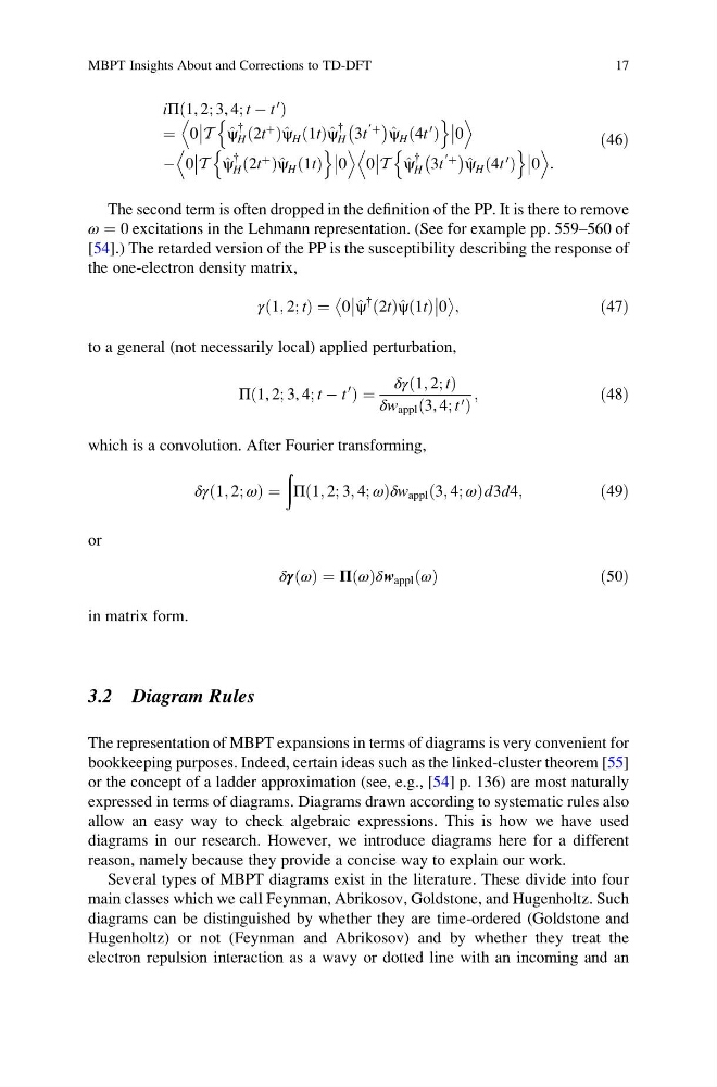
iΠ 1, 2; 3, 4; t À t
0
ð
Þ
¼ 0
T ^
ψ
{
H 2t
þ
ð Þ^ ψ H 1t
ð Þ^ ψ
{
H 3t
0 þ
À
Á ^
ψ H 4t
0
ð Þ
n
o
0
D
E
À 0
T ^
ψ
{
H 2t
þ
ð Þ^ ψ H 1t
ð Þ
n
o
0
D
E
0
T ^
ψ
{
H 3t
0 þ
À
Á ^
ψ H 4t
0
ð Þ
n
o
0
D
E
:
ð46Þ
The second term is often dropped in the definition of the PP. It is there to remove
ω ¼ 0 excitations in the Lehmann representation. (See for example pp. 559–560 of
[54].) The retarded version of the PP is the susceptibility describing the response of
the one-electron density matrix,
γ 1; 2; t
ð
Þ¼ 0
^
ψ
{ 2t
ð Þ^ ψ 1t
ð Þ
0
;
ð47Þ
to a general (not necessarily local) applied perturbation,
Π 1, 2; 3, 4; t À t
0
ð
Þ ¼
δγ 1; 2; t
ð
Þ
δw appl ð3, 4; t 0 Þ
;
ð48Þ
which is a convolution. After Fourier transforming,
δγ 1; 2; ω
ð
Þ¼
ð
Π 1; 2; 3; 4; ω
ð
Þ δw appl 3; 4; ω
ð
Þd3d4;
ð49Þ
or
δγ ω
ð Þ ¼ Π ω
ð Þδw appl ω
ð Þ
ð50Þ
in matrix form.
3.2 Diagram Rules
The representation of MBPT expansions in terms of diagrams is very convenient for
bookkeeping purposes. Indeed, certain ideas such as the linked-cluster theorem [55]
or the concept of a ladder approximation (see, e.g., [54] p. 136) are most naturally
expressed in terms of diagrams. Diagrams drawn according to systematic rules also
allow an easy way to check algebraic expressions. This is how we have used
diagrams in our research. However, we introduce diagrams here for a different
reason, namely because they provide a concise way to explain our work.
Several types of MBPT diagrams exist in the literature. These divide into four
main classes which we call Feynman, Abrikosov, Goldstone, and Hugenholtz. Such
diagrams can be distinguished by whether they are time-ordered (Goldstone and
Hugenholtz) or not (Feynman and Abrikosov) and by whether they treat the
electron repulsion interaction as a wavy or dotted line with an incoming and an
MBPT Insights About and Corrections to TD-DFT
17
0
ð
Þ
¼ 0
T ^
ψ
{
H 2t
þ
ð Þ^ ψ H 1t
ð Þ^ ψ
{
H 3t
0 þ
À
Á ^
ψ H 4t
0
ð Þ
n
o
0
D
E
À 0
T ^
ψ
{
H 2t
þ
ð Þ^ ψ H 1t
ð Þ
n
o
0
D
E
0
T ^
ψ
{
H 3t
0 þ
À
Á ^
ψ H 4t
0
ð Þ
n
o
0
D
E
:
ð46Þ
The second term is often dropped in the definition of the PP. It is there to remove
ω ¼ 0 excitations in the Lehmann representation. (See for example pp. 559–560 of
[54].) The retarded version of the PP is the susceptibility describing the response of
the one-electron density matrix,
γ 1; 2; t
ð
Þ¼ 0
^
ψ
{ 2t
ð Þ^ ψ 1t
ð Þ
0
;
ð47Þ
to a general (not necessarily local) applied perturbation,
Π 1, 2; 3, 4; t À t
0
ð
Þ ¼
δγ 1; 2; t
ð
Þ
δw appl ð3, 4; t 0 Þ
;
ð48Þ
which is a convolution. After Fourier transforming,
δγ 1; 2; ω
ð
Þ¼
ð
Π 1; 2; 3; 4; ω
ð
Þ δw appl 3; 4; ω
ð
Þd3d4;
ð49Þ
or
δγ ω
ð Þ ¼ Π ω
ð Þδw appl ω
ð Þ
ð50Þ
in matrix form.
3.2 Diagram Rules
The representation of MBPT expansions in terms of diagrams is very convenient for
bookkeeping purposes. Indeed, certain ideas such as the linked-cluster theorem [55]
or the concept of a ladder approximation (see, e.g., [54] p. 136) are most naturally
expressed in terms of diagrams. Diagrams drawn according to systematic rules also
allow an easy way to check algebraic expressions. This is how we have used
diagrams in our research. However, we introduce diagrams here for a different
reason, namely because they provide a concise way to explain our work.
Several types of MBPT diagrams exist in the literature. These divide into four
main classes which we call Feynman, Abrikosov, Goldstone, and Hugenholtz. Such
diagrams can be distinguished by whether they are time-ordered (Goldstone and
Hugenholtz) or not (Feynman and Abrikosov) and by whether they treat the
electron repulsion interaction as a wavy or dotted line with an incoming and an
MBPT Insights About and Corrections to TD-DFT
17