

α p, g 0 g
00 i
X
e
V g 0 e V eg
00
ð 1
À1
dτ 2
ð τ 2
À1
dτ 1 ℰ
*
p τ 2
ð Þℰ p τ 1
ð Þe
i ω p Àω eg 0 þiγ e
ð
Þ τ 2 Ài
À
ω p Àω eg
00 þiγ e
Á
τ 1
:
ð18Þ
Here, ω ev is the frequency for the v ! e transition, and γ e is the inverse of the
excitation lifetime. In some applications, it may be more convenient to work in the
frequency domain where the spectral (rather than temporal) field envelopes are
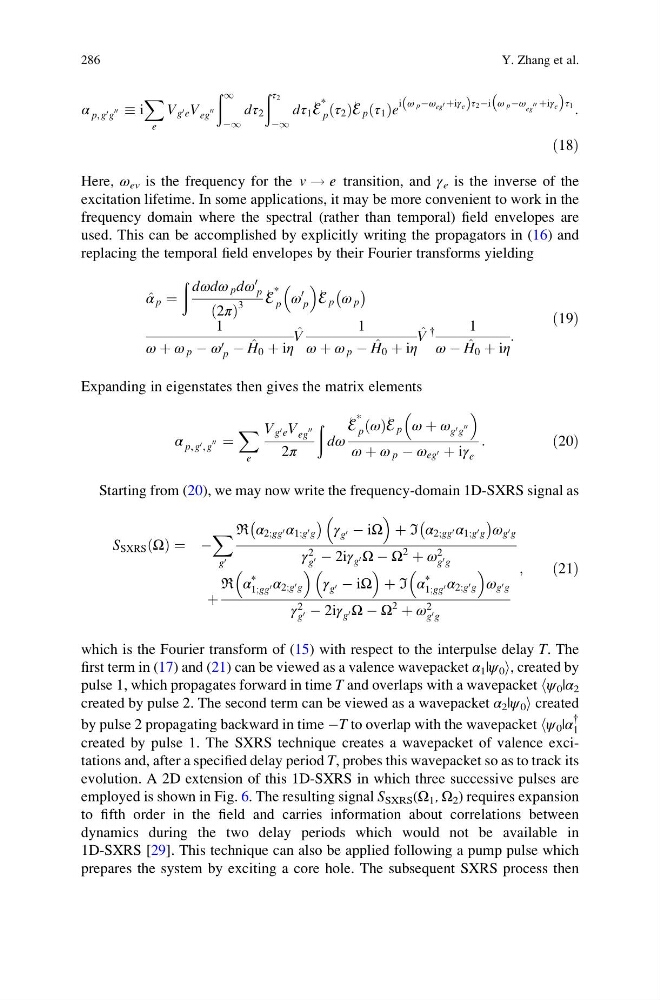
used. This can be accomplished by explicitly writing the propagators in (16) and
replacing the temporal field envelopes by their Fourier transforms yielding
^
α p ¼
ð dωdω p dω
0
p
2π
ð Þ
3
ℰ
*
p ω
0
p
ℰ p ω p
À Á
1
ω þ ω p À ω 0
p À ^
H 0 þ iη
^
V
1
ω þ ω p À ^
H 0 þ iη
^
V
{
1
ω À ^
H 0 þ iη
:
ð19Þ
Expanding in eigenstates then gives the matrix elements
α p, g 0 , g
00 ¼
X
e
V g 0 e V eg
00
2π
ð
dω
ℰ
*
p ω
ð Þℰ p ω þ ω g 0 g
00
ω þ ω p À ω eg 0 þ iγ e
:
ð20Þ
Starting from (20), we may now write the frequency-domain 1D-SXRS signal as
S SXRS Ω
ð Þ ¼ À
X
g 0
ℜ α 2;gg 0 α 1;g 0 g
À
Á γ g 0 À iΩ
þ ℑ α 2;gg 0 α 1;g 0 g
À
Á ω g 0 g
γ 2
g 0 À 2iγ g 0 Ω À Ω
2
þ ω 2
g 0 g
þ
ℜ α
*
1;gg 0 α 2;g 0 g
γ g 0 À iΩ
þ ℑ α
*
1;gg 0 α 2;g 0 g
ω g 0 g
γ 2
g 0 À 2iγ g 0 Ω À Ω
2
þ ω 2
g 0 g
;
ð21Þ
which is the Fourier transform of (15) with respect to the interpulse delay T. The
first term in (17) and (21) can be viewed as a valence wavepacket α 1 |ψ 0 i, created by
pulse 1, which propagates forward in time T and overlaps with a wavepacket hψ 0 |α 2
created by pulse 2. The second term can be viewed as a wavepacket α 2 |ψ 0 i created
by pulse 2 propagating backward in time ÀT to overlap with the wavepacket hψ 0 |α
{
1
created by pulse 1. The SXRS technique creates a wavepacket of valence excitations and, after a specified delay period T, probes this wavepacket so as to track its
evolution. A 2D extension of this 1D-SXRS in which three successive pulses are
employed is shown in Fig. 6. The resulting signal S SXRS (Ω 1 , Ω 2 ) requires expansion
to fifth order in the field and carries information about correlations between
dynamics during the two delay periods which would not be available in
1D-SXRS [29]. This technique can also be applied following a pump pulse which
prepares the system by exciting a core hole. The subsequent SXRS process then
286
Y. Zhang et al.
00 i
X
e
V g 0 e V eg
00
ð 1
À1
dτ 2
ð τ 2
À1
dτ 1 ℰ
*
p τ 2
ð Þℰ p τ 1
ð Þe
i ω p Àω eg 0 þiγ e
ð
Þ τ 2 Ài
À
ω p Àω eg
00 þiγ e
Á
τ 1
:
ð18Þ
Here, ω ev is the frequency for the v ! e transition, and γ e is the inverse of the
excitation lifetime. In some applications, it may be more convenient to work in the
frequency domain where the spectral (rather than temporal) field envelopes are
used. This can be accomplished by explicitly writing the propagators in (16) and
replacing the temporal field envelopes by their Fourier transforms yielding
^
α p ¼
ð dωdω p dω
0
p
2π
ð Þ
3
ℰ
*
p ω
0
p
ℰ p ω p
À Á
1
ω þ ω p À ω 0
p À ^
H 0 þ iη
^
V
1
ω þ ω p À ^
H 0 þ iη
^
V
{
1
ω À ^
H 0 þ iη
:
ð19Þ
Expanding in eigenstates then gives the matrix elements
α p, g 0 , g
00 ¼
X
e
V g 0 e V eg
00
2π
ð
dω
ℰ
*
p ω
ð Þℰ p ω þ ω g 0 g
00
ω þ ω p À ω eg 0 þ iγ e
:
ð20Þ
Starting from (20), we may now write the frequency-domain 1D-SXRS signal as
S SXRS Ω
ð Þ ¼ À
X
g 0
ℜ α 2;gg 0 α 1;g 0 g
À
Á γ g 0 À iΩ
þ ℑ α 2;gg 0 α 1;g 0 g
À
Á ω g 0 g
γ 2
g 0 À 2iγ g 0 Ω À Ω
2
þ ω 2
g 0 g
þ
ℜ α
*
1;gg 0 α 2;g 0 g
γ g 0 À iΩ
þ ℑ α
*
1;gg 0 α 2;g 0 g
ω g 0 g
γ 2
g 0 À 2iγ g 0 Ω À Ω
2
þ ω 2
g 0 g
;
ð21Þ
which is the Fourier transform of (15) with respect to the interpulse delay T. The
first term in (17) and (21) can be viewed as a valence wavepacket α 1 |ψ 0 i, created by
pulse 1, which propagates forward in time T and overlaps with a wavepacket hψ 0 |α 2
created by pulse 2. The second term can be viewed as a wavepacket α 2 |ψ 0 i created
by pulse 2 propagating backward in time ÀT to overlap with the wavepacket hψ 0 |α
{
1
created by pulse 1. The SXRS technique creates a wavepacket of valence excitations and, after a specified delay period T, probes this wavepacket so as to track its
evolution. A 2D extension of this 1D-SXRS in which three successive pulses are
employed is shown in Fig. 6. The resulting signal S SXRS (Ω 1 , Ω 2 ) requires expansion
to fifth order in the field and carries information about correlations between
dynamics during the two delay periods which would not be available in
1D-SXRS [29]. This technique can also be applied following a pump pulse which
prepares the system by exciting a core hole. The subsequent SXRS process then
286
Y. Zhang et al.