

S SXRS Λ
ð Þ ¼ ℑ
ð
dτ 4
ð τ 4
À1
dτ 3
ð τ 3
À1
dτ 2
ð τ 2
À1
dτ 1 i
ð Þ
3 ℰ
*
2 τ 4
ð Þℰ τ 3
ð Þ
 ℰ
*
1 τ 2
ð Þℰ 1 τ 1
ð Þ ψ 0 ^
V τ 4
ð Þ ^
V
{
τ 3
ð Þ ^
V τ 2
ð Þ ^
V
{
τ 1
ð Þ
ψ 0
h
þ ℰ 1 τ 2
ð Þℰ
*
1 τ 1
ð Þ ψ 0 ^
V
{
τ 1
ð Þ ^
V τ 2
ð Þ ^
V τ 4
ð Þ ^
V
{
τ 3
ð Þ
ψ 0
i
:
ð15Þ
Because the interactions are paired within a given pulse and the pulses are temporally well-separated, we may extend the upper limit for the τ 2 integration to infinity.
This permits us to define formally the polarizability ^
α p induced by the pth pulse:
^
α p Λ p
À Á i
ð 1
À1
dτ
ð τ
À1
dτ
0 ^
V τ
ð Þ ^
V
{
τ
0
ð Þℰ
*
p τ
ð Þℰ p τ
0
ð Þ;
ð16Þ
which is both a material operator and a function of Λ p , the parameters of the pth
pulse. In the limit of ultrashort pulses, the primary Λ p parameter is the central pulse
time τ p and the principal control variable for the 1D-SXRS signal is the interpulse
delay T ¼ τ 2 À τ 1 and the signal is recast as
S T
ð Þ ¼ ℜ ^
α 2 T
ð Þ^ α 1 0
ð Þ
h
iþ ^
α
*
1 0
ð Þ^ α 2 T
ð Þ
Â
à ;
ð17Þ
where we have set τ 1 ¼ 0 as the origin of time. Taking matrix elements in the
Hamiltonian eigenbasis gives the sum-over-states expression
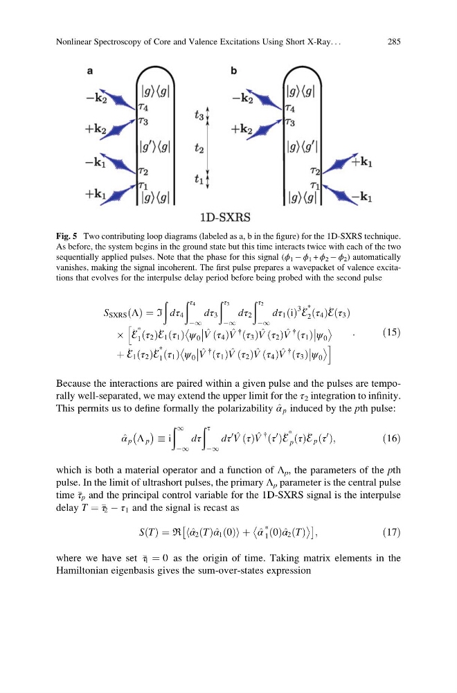
Fig. 5 Two contributing loop diagrams (labeled as a, b in the figure) for the 1D-SXRS technique.
As before, the system begins in the ground state but this time interacts twice with each of the two
sequentially applied pulses. Note that the phase for this signal (ϕ 1 À ϕ 1 + ϕ 2 À ϕ 2 ) automatically
vanishes, making the signal incoherent. The first pulse prepares a wavepacket of valence excitations that evolves for the interpulse delay period before being probed with the second pulse
Nonlinear Spectroscopy of Core and Valence Excitations Using Short X-Ray. . .
285
ð Þ ¼ ℑ
ð
dτ 4
ð τ 4
À1
dτ 3
ð τ 3
À1
dτ 2
ð τ 2
À1
dτ 1 i
ð Þ
3 ℰ
*
2 τ 4
ð Þℰ τ 3
ð Þ
 ℰ
*
1 τ 2
ð Þℰ 1 τ 1
ð Þ ψ 0 ^
V τ 4
ð Þ ^
V
{
τ 3
ð Þ ^
V τ 2
ð Þ ^
V
{
τ 1
ð Þ
ψ 0
h
þ ℰ 1 τ 2
ð Þℰ
*
1 τ 1
ð Þ ψ 0 ^
V
{
τ 1
ð Þ ^
V τ 2
ð Þ ^
V τ 4
ð Þ ^
V
{
τ 3
ð Þ
ψ 0
i
:
ð15Þ
Because the interactions are paired within a given pulse and the pulses are temporally well-separated, we may extend the upper limit for the τ 2 integration to infinity.
This permits us to define formally the polarizability ^
α p induced by the pth pulse:
^
α p Λ p
À Á i
ð 1
À1
dτ
ð τ
À1
dτ
0 ^
V τ
ð Þ ^
V
{
τ
0
ð Þℰ
*
p τ
ð Þℰ p τ
0
ð Þ;
ð16Þ
which is both a material operator and a function of Λ p , the parameters of the pth
pulse. In the limit of ultrashort pulses, the primary Λ p parameter is the central pulse
time τ p and the principal control variable for the 1D-SXRS signal is the interpulse
delay T ¼ τ 2 À τ 1 and the signal is recast as
S T
ð Þ ¼ ℜ ^
α 2 T
ð Þ^ α 1 0
ð Þ
h
iþ ^
α
*
1 0
ð Þ^ α 2 T
ð Þ
Â
à ;
ð17Þ
where we have set τ 1 ¼ 0 as the origin of time. Taking matrix elements in the
Hamiltonian eigenbasis gives the sum-over-states expression
Fig. 5 Two contributing loop diagrams (labeled as a, b in the figure) for the 1D-SXRS technique.
As before, the system begins in the ground state but this time interacts twice with each of the two
sequentially applied pulses. Note that the phase for this signal (ϕ 1 À ϕ 1 + ϕ 2 À ϕ 2 ) automatically
vanishes, making the signal incoherent. The first pulse prepares a wavepacket of valence excitations that evolves for the interpulse delay period before being probed with the second pulse
Nonlinear Spectroscopy of Core and Valence Excitations Using Short X-Ray. . .
285