

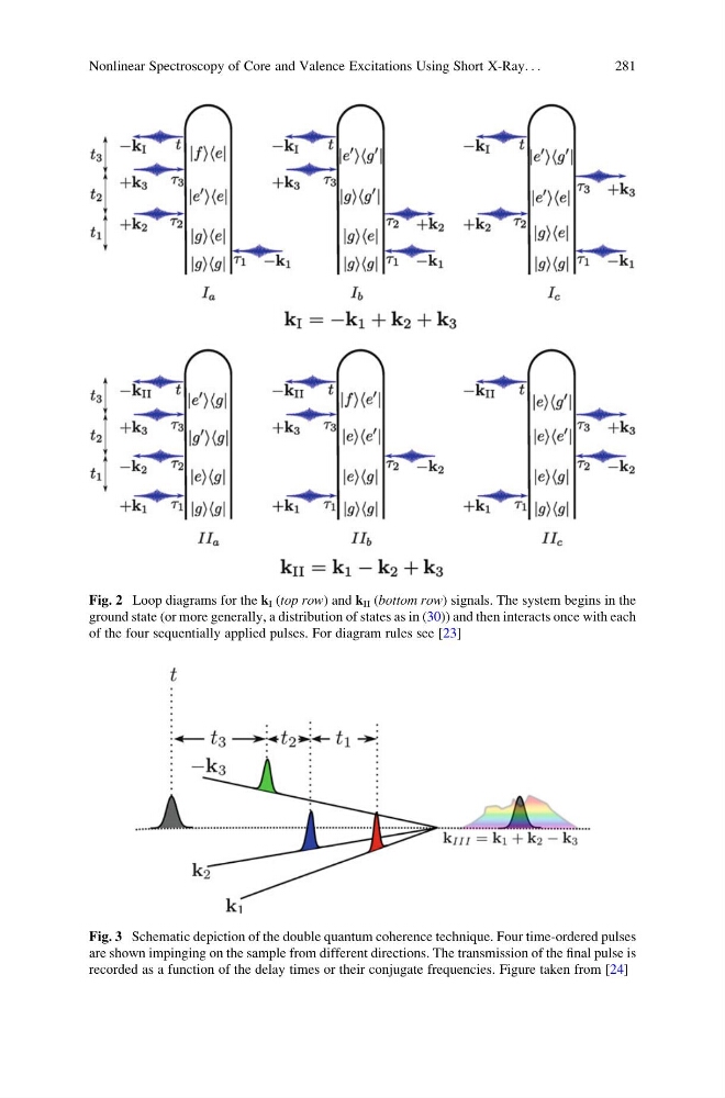
Fig. 2 Loop diagrams for the k I (top row) and k II (bottom row) signals. The system begins in the
ground state (or more generally, a distribution of states as in (30)) and then interacts once with each
of the four sequentially applied pulses. For diagram rules see [23]
Fig. 3 Schematic depiction of the double quantum coherence technique. Four time-ordered pulses
are shown impinging on the sample from different directions. The transmission of the final pulse is
recorded as a function of the delay times or their conjugate frequencies. Figure taken from [24]
Nonlinear Spectroscopy of Core and Valence Excitations Using Short X-Ray. . .
281
ground state (or more generally, a distribution of states as in (30)) and then interacts once with each
of the four sequentially applied pulses. For diagram rules see [23]
Fig. 3 Schematic depiction of the double quantum coherence technique. Four time-ordered pulses
are shown impinging on the sample from different directions. The transmission of the final pulse is
recorded as a function of the delay times or their conjugate frequencies. Figure taken from [24]
Nonlinear Spectroscopy of Core and Valence Excitations Using Short X-Ray. . .
281