

In the remainder of this chapter we first show how MBPT may be used to derive
expressions for the A
CI
1, 2þ , A
CI
2þ, 1 , and A
CI
2þ, 2þ blocks and show how this may be used
in the form of dressed TD-DFT to correct the AA. Then we discuss localization of
the terms beyond the AA in order to obtain some insight into the analytic behavior
of the xc-kernel.
3 Many-Body Perturbation Theory (MBPT)
This section elaborates on the polarization propagator (PP) approach. As the PP was
originally inspired by the Bethe–Salpeter equation (BSE) and as the BSE often
crops up in articles from the solid-state physics community which are concerned
with both TD-DFT and MBPT [41–47], we try to make the connection between the
PP and BSE approaches as clear as possible. Although the two MBPT approaches
are formally equivalent, differences emerge because the BSE approach emphasizes
the time representation whereas the PP approach emphasizes the frequency representation. This can and typically does lead to different approximations. In particular, it seems to be easier to derive pole structure-conserving approximations
needed for treating two-electron and higher excitations in the frequency representation than in the time representation. This and prior experience with the PP
approach in the quantum chemistry community [48–53] have led us to favor the
PP approach. We make extensive use of diagrams in order to give an overview of
our manipulations. Whenever possible, more elaborate mathematical manipulations
are relegated to the appendix.
3.1 Green’s Functions
Perhaps the most common and arguably the most basic quantity in MBPT is the
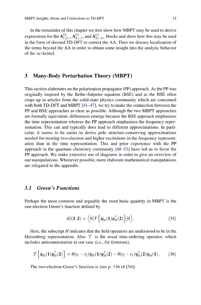
one-electron Green’s function defined by
iG 1; 2
ð Þ ¼ 0
T ^
ψ H 1
ð Þ^ ψ
{
H 2
ð Þ
n
o
0
D
E
:
ð35Þ
Here, the subscript H indicates that the field operators are understood to be in the
Heisenberg representation. Also T is the usual time-ordering operator, which
includes anticommutation in our case (i.e., for fermions),
T ^
ψ H 1
ð Þ^ ψ
{
H 2
ð Þ
n
o
¼ θ t 1 À t 2
ð
Þ^ ψ H 1
ð Þ^ ψ
{
H 2
ð Þ À θ t 2 À t 1
ð
Þ^ ψ
{
H 2
ð Þ^ ψ H 1
ð Þ:
ð36Þ
The two-electron Green’s function is (see p. 116 of [54])
MBPT Insights About and Corrections to TD-DFT
15
expressions for the A
CI
1, 2þ , A
CI
2þ, 1 , and A
CI
2þ, 2þ blocks and show how this may be used
in the form of dressed TD-DFT to correct the AA. Then we discuss localization of
the terms beyond the AA in order to obtain some insight into the analytic behavior
of the xc-kernel.
3 Many-Body Perturbation Theory (MBPT)
This section elaborates on the polarization propagator (PP) approach. As the PP was
originally inspired by the Bethe–Salpeter equation (BSE) and as the BSE often
crops up in articles from the solid-state physics community which are concerned
with both TD-DFT and MBPT [41–47], we try to make the connection between the
PP and BSE approaches as clear as possible. Although the two MBPT approaches
are formally equivalent, differences emerge because the BSE approach emphasizes
the time representation whereas the PP approach emphasizes the frequency representation. This can and typically does lead to different approximations. In particular, it seems to be easier to derive pole structure-conserving approximations
needed for treating two-electron and higher excitations in the frequency representation than in the time representation. This and prior experience with the PP
approach in the quantum chemistry community [48–53] have led us to favor the
PP approach. We make extensive use of diagrams in order to give an overview of
our manipulations. Whenever possible, more elaborate mathematical manipulations
are relegated to the appendix.
3.1 Green’s Functions
Perhaps the most common and arguably the most basic quantity in MBPT is the
one-electron Green’s function defined by
iG 1; 2
ð Þ ¼ 0
T ^
ψ H 1
ð Þ^ ψ
{
H 2
ð Þ
n
o
0
D
E
:
ð35Þ
Here, the subscript H indicates that the field operators are understood to be in the
Heisenberg representation. Also T is the usual time-ordering operator, which
includes anticommutation in our case (i.e., for fermions),
T ^
ψ H 1
ð Þ^ ψ
{
H 2
ð Þ
n
o
¼ θ t 1 À t 2
ð
Þ^ ψ H 1
ð Þ^ ψ
{
H 2
ð Þ À θ t 2 À t 1
ð
Þ^ ψ
{
H 2
ð Þ^ ψ H 1
ð Þ:
ð36Þ
The two-electron Green’s function is (see p. 116 of [54])
MBPT Insights About and Corrections to TD-DFT
15