

^
H t
ð Þ ¼ ^
H v t
ð Þ for r
j j ! r s and all t;
ð79Þ
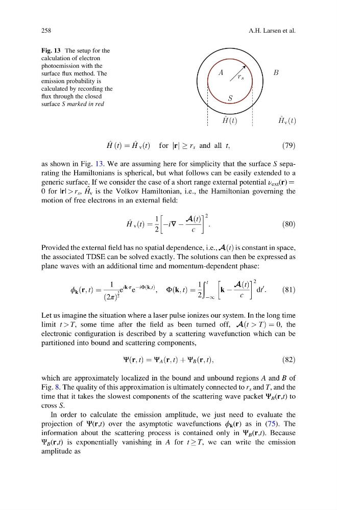
as shown in Fig. 13. We are assuming here for simplicity that the surface S separating the Hamiltonians is spherical, but what follows can be easily extended to a
generic surface. If we consider the case of a short range external potential ν ext (r) ¼
0 for |r| > r s , H ˆ
v is the Volkov Hamiltonian, i.e., the Hamiltonian governing the
motion of free electrons in an external field:
^
H v t
ð Þ ¼
1
2
Ài∇ À
A t
ð Þ
c
! 2
:
ð80Þ
Provided the external field has no spatial dependence, i.e., A t
ð Þ is constant in space,
the associated TDSE can be solved exactly. The solutions can then be expressed as
plane waves with an additional time and momentum-dependent phase:
ϕ k r; t
ð Þ ¼
1
2π
ð Þ
3
2
e
ikÁr e
ÀiΦ k;t
ð Þ , Φ k; t
ð Þ ¼
1
2
ð t
À1
k À
A t
ð Þ
c
! 2
dt
0
:
ð81Þ
Let us imagine the situation where a laser pulse ionizes our system. In the long time
limit t > T, some time after the field as been turned off, A t > T
ð
Þ¼0, the
electronic configuration is described by a scattering wavefunction which can be
partitioned into bound and scattering components,
Ψ r; t
ð Þ ¼ Ψ A r; t
ð Þ þ Ψ B r; t
ð Þ;
ð82Þ
which are approximately localized in the bound and unbound regions A and B of
Fig. 8. The quality of this approximation is ultimately connected to r s and T, and the
time that it takes the slowest components of the scattering wave packet Ψ B (r,t) to
cross S.
In order to calculate the emission amplitude, we just need to evaluate the
projection of Ψ(r,t) over the asymptotic wavefunctions ϕ k (r) as in (75). The
information about the scattering process is contained only in Ψ B (r,t). Because
Ψ B (r,t) is exponentially vanishing in A for t ! T, we can write the emission
amplitude as
Fig. 13 The setup for the
calculation of electron
photoemission with the
surface flux method. The
emission probability is
calculated by recording the
flux through the closed
surface S marked in red
258
A.H. Larsen et al.
H t
ð Þ ¼ ^
H v t
ð Þ for r
j j ! r s and all t;
ð79Þ
as shown in Fig. 13. We are assuming here for simplicity that the surface S separating the Hamiltonians is spherical, but what follows can be easily extended to a
generic surface. If we consider the case of a short range external potential ν ext (r) ¼
0 for |r| > r s , H ˆ
v is the Volkov Hamiltonian, i.e., the Hamiltonian governing the
motion of free electrons in an external field:
^
H v t
ð Þ ¼
1
2
Ài∇ À
A t
ð Þ
c
! 2
:
ð80Þ
Provided the external field has no spatial dependence, i.e., A t
ð Þ is constant in space,
the associated TDSE can be solved exactly. The solutions can then be expressed as
plane waves with an additional time and momentum-dependent phase:
ϕ k r; t
ð Þ ¼
1
2π
ð Þ
3
2
e
ikÁr e
ÀiΦ k;t
ð Þ , Φ k; t
ð Þ ¼
1
2
ð t
À1
k À
A t
ð Þ
c
! 2
dt
0
:
ð81Þ
Let us imagine the situation where a laser pulse ionizes our system. In the long time
limit t > T, some time after the field as been turned off, A t > T
ð
Þ¼0, the
electronic configuration is described by a scattering wavefunction which can be
partitioned into bound and scattering components,
Ψ r; t
ð Þ ¼ Ψ A r; t
ð Þ þ Ψ B r; t
ð Þ;
ð82Þ
which are approximately localized in the bound and unbound regions A and B of
Fig. 8. The quality of this approximation is ultimately connected to r s and T, and the
time that it takes the slowest components of the scattering wave packet Ψ B (r,t) to
cross S.
In order to calculate the emission amplitude, we just need to evaluate the
projection of Ψ(r,t) over the asymptotic wavefunctions ϕ k (r) as in (75). The
information about the scattering process is contained only in Ψ B (r,t). Because
Ψ B (r,t) is exponentially vanishing in A for t ! T, we can write the emission
amplitude as
Fig. 13 The setup for the
calculation of electron
photoemission with the
surface flux method. The
emission probability is
calculated by recording the
flux through the closed
surface S marked in red
258
A.H. Larsen et al.