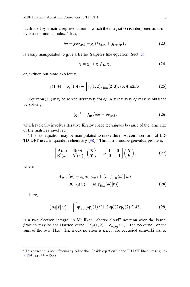
facilitated by a matrix representation in which the integration is interpreted as a sum
over a continuous index. Thus,
δρ ¼ χ δv appl ¼ χ s δv appl þ f Hxc δρ
À
Á ;
ð23Þ
is easily manipulated to give a Bethe–Salpeter-like equation (Sect. 3),
χ ¼ χ s þ χ s f Hxc χ ;
ð24Þ
or, written out more explicitly,
χ 1; 4
ð Þ ¼ χ s 1; 4
ð Þþ
ð
χ s 1; 2
ð Þf Hxc 2; 3
ð Þχ 3; 4
ð Þd2d3 :
ð25Þ
Equation (23) may be solved iteratively for δρ. Alternatively δρ may be obtained
by solving
χ
À1
s À f Hxc
À
Á δρ ¼ δv appl ;
ð26Þ
which typically involves iterative Krylov space techniques because of the large size
of the matrices involved.
This last equation may be manipulated to make the most common form of LRTD-DFT used in quantum chemistry [38].
5 This is a pseudoeigenvalue problem,
A ω
ð Þ B ω
ð Þ
B
*
ω
ð Þ A
*
ω
ð Þ
!
X
Y
¼ ω
1 0
0 À1
!
X
Y
;
ð27Þ
where
A ia, jb ω
ð Þ ¼ δ i, j δ a, b ε a, i þ ia
f Hxc ω
ð Þ
jb
À
Á
B ia, b j ω
ð Þ ¼ ia
f Hxc ω
ð Þ
b j
À
Á :
ð28Þ
Here,
pq
f
rs
À
Á ¼
ðð
ψ
*
p 1
ð Þψ q 1
ð Þf 1; 2
ð Þψ
*
r 2
ð Þψ s 2
ð Þd1d2 ;
ð29Þ
is a two electron integral in Mulliken “charge-cloud” notation over the kernel
f which may be the Hartree kernel [ f H 1; 2
ð Þ ¼ δ σ 1 , σ 2 =r 12 ], the xc-kernel, or the
sum of the two (Hxc). The index notation is i, j, . . . for occupied spin-orbitals, a,
5 This equation is not infrequently called the “Casida equation” in the TD-DFT literature (e.g., as
in [24], pp. 145–153.)
MBPT Insights About and Corrections to TD-DFT
13