2.3 Linear Response (LR-) TD-DFT
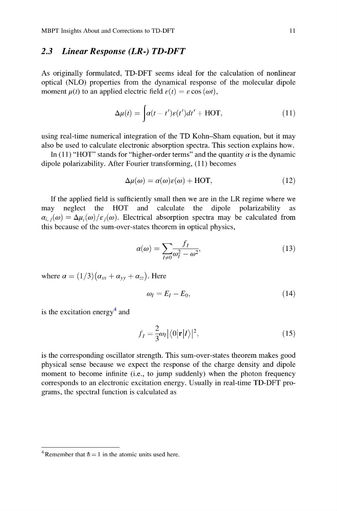
As originally formulated, TD-DFT seems ideal for the calculation of nonlinear
optical (NLO) properties from the dynamical response of the molecular dipole
moment μ(t) to an applied electric field ε t
ð Þ ¼ ε cos ωt
ð Þ,
Δμ t
ð Þ ¼
ð
α t À t
0
ð
Þε t
0
ð Þdt
0
þ HOT;
ð11Þ
using real-time numerical integration of the TD Kohn–Sham equation, but it may
also be used to calculate electronic absorption spectra. This section explains how.
In (11) “HOT” stands for “higher-order terms” and the quantity α is the dynamic
dipole polarizability. After Fourier transforming, (11) becomes
Δμ ω
ð Þ ¼ α ω
ð Þε ω
ð Þ þ HOT;
ð12Þ
If the applied field is sufficiently small then we are in the LR regime where we
may neglect the HOT and calculate the dipole polarizability as
α i, j ω
ð Þ ¼ Δμ i ω
ð Þ=ε j ω
ð Þ. Electrical absorption spectra may be calculated from
this because of the sum-over-states theorem in optical physics,
α ω
ð Þ ¼
X
I6 ¼0
f I
ω 2
I À ω 2 ;
ð13Þ
where α ¼ 1=3
ð
Þ α xx þ α yy þ α zz
À
Á
. Here
ω I ¼ E I À E 0 ;
ð14Þ
is the excitation energy
4 and
f I ¼
2
3
ω I
0
r
I
2 ;
ð15Þ
is the corresponding oscillator strength. This sum-over-states theorem makes good
physical sense because we expect the response of the charge density and dipole
moment to become infinite (i.e., to jump suddenly) when the photon frequency
corresponds to an electronic excitation energy. Usually in real-time TD-DFT programs, the spectral function is calculated as
4 Remember that h ¼ 1 in the atomic units used here.
MBPT Insights About and Corrections to TD-DFT
11