

but systematically occurs in bulk insulators and semiconductors. The underlying
reason is the long-range behavior of the xc kernel: in reciprocal space, the head of
f xc should diverge as 1/q
2 for small q, but semilocal approximations instead
approach a constant. In the next sections we explain this in more detail.
The main reason why excitons in TDDFT are a hard problem is thus that the
standard local and semilocal xc kernels don’t work, and one needs to resort to
nonstandard kernels or even develop new ones. We discuss this in Sect. 5.4 and
show some results.
Another reason is of a more practical nature. Even if very good approximations
for the xc kernel are available, the calculations can be numerically difficult because
convergence in reciprocal space can be slow. This problem also affects the standard
many-body approaches (GW-BSE) [76, 77].
5.2 Formalism: Direct Calculation of Exciton Binding
Energies
The Kohn–Sham response function χ s has poles at the single-particle Kohn–Sham
excitation energies, which can be clearly seen in (25) and (29). On the other hand,
the full many-body response function χ has poles at the exact excitation energies of
the system [1, 71]. This is true for any type of system, finite or extended. The
Hartree and xc kernels in (24) and (28) are responsible for transforming the Kohn–
Sham excitation spectrum into the exact one; this includes the creation of excitations which have no counterpart in the Kohn–Sham spectrum, such as plasmons in
metals or excitons in semiconductors and insulators.
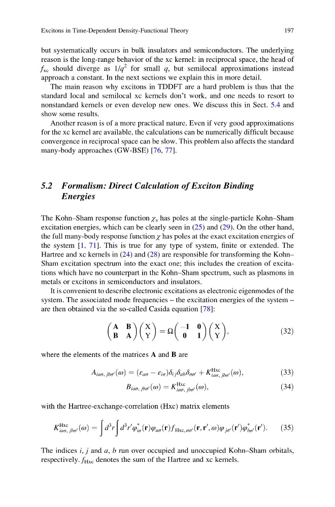
It is convenient to describe electronic excitations as electronic eigenmodes of the
system. The associated mode frequencies – the excitation energies of the system –
are then obtained via the so-called Casida equation [78]:
A B
B A
X
Y
¼ Ω
À1 0
0 1
X
Y
;
ð32Þ
where the elements of the matrices A and B are
A iaσ, jbσ 0 ω
ð Þ ¼ ε aσ À ε iσ
ð
Þ δ i j δ ab δ σσ 0 þ K
Hxc
iaσ, jbσ 0 ω
ð Þ;
ð33Þ
B iaσ, jbσ 0 ω
ð Þ ¼ K
Hxc
iaσ, jbσ 0 ω
ð Þ;
ð34Þ
with the Hartree-exchange-correlation (Hxc) matrix elements
K
Hxc
iaσ, jbσ 0 ω
ð Þ ¼
ð
d
3 r
ð
d
3 r
0
φ
*
iσ r
ð Þφ aσ r
ð Þ f Hxc, σσ 0 ðr, r
0 , ωÞφ jσ 0 r
0
ð Þφ
*
bσ 0 r
0
ð Þ:
ð35Þ
The indices i, j and a, b run over occupied and unoccupied Kohn–Sham orbitals,
respectively. f Hxc denotes the sum of the Hartree and xc kernels.
Excitons in Time-Dependent Density-Functional Theory
197
reason is the long-range behavior of the xc kernel: in reciprocal space, the head of
f xc should diverge as 1/q
2 for small q, but semilocal approximations instead
approach a constant. In the next sections we explain this in more detail.
The main reason why excitons in TDDFT are a hard problem is thus that the
standard local and semilocal xc kernels don’t work, and one needs to resort to
nonstandard kernels or even develop new ones. We discuss this in Sect. 5.4 and
show some results.
Another reason is of a more practical nature. Even if very good approximations
for the xc kernel are available, the calculations can be numerically difficult because
convergence in reciprocal space can be slow. This problem also affects the standard
many-body approaches (GW-BSE) [76, 77].
5.2 Formalism: Direct Calculation of Exciton Binding
Energies
The Kohn–Sham response function χ s has poles at the single-particle Kohn–Sham
excitation energies, which can be clearly seen in (25) and (29). On the other hand,
the full many-body response function χ has poles at the exact excitation energies of
the system [1, 71]. This is true for any type of system, finite or extended. The
Hartree and xc kernels in (24) and (28) are responsible for transforming the Kohn–
Sham excitation spectrum into the exact one; this includes the creation of excitations which have no counterpart in the Kohn–Sham spectrum, such as plasmons in
metals or excitons in semiconductors and insulators.
It is convenient to describe electronic excitations as electronic eigenmodes of the
system. The associated mode frequencies – the excitation energies of the system –
are then obtained via the so-called Casida equation [78]:
A B
B A
X
Y
¼ Ω
À1 0
0 1
X
Y
;
ð32Þ
where the elements of the matrices A and B are
A iaσ, jbσ 0 ω
ð Þ ¼ ε aσ À ε iσ
ð
Þ δ i j δ ab δ σσ 0 þ K
Hxc
iaσ, jbσ 0 ω
ð Þ;
ð33Þ
B iaσ, jbσ 0 ω
ð Þ ¼ K
Hxc
iaσ, jbσ 0 ω
ð Þ;
ð34Þ
with the Hartree-exchange-correlation (Hxc) matrix elements
K
Hxc
iaσ, jbσ 0 ω
ð Þ ¼
ð
d
3 r
ð
d
3 r
0
φ
*
iσ r
ð Þφ aσ r
ð Þ f Hxc, σσ 0 ðr, r
0 , ωÞφ jσ 0 r
0
ð Þφ
*
bσ 0 r
0
ð Þ:
ð35Þ
The indices i, j and a, b run over occupied and unoccupied Kohn–Sham orbitals,
respectively. f Hxc denotes the sum of the Hartree and xc kernels.
Excitons in Time-Dependent Density-Functional Theory
197