

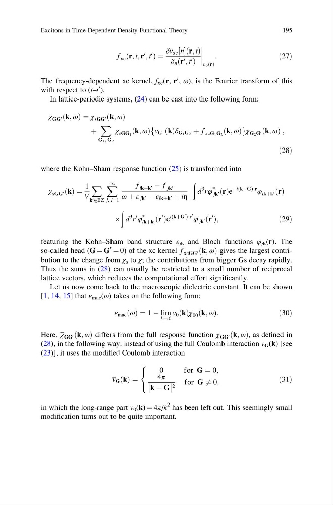
f xc r, t, r
0 , t
0
ð
Þ¼
δv xc n
½ r; t
ð Þ
δ n r 0 ; t 0
ð
Þ
n 0 r
ð Þ
:
ð27Þ
The frequency-dependent xc kernel, f xc (r, r
0 , ω), is the Fourier transform of this
with respect to (t–t
0 ).
In lattice-periodic systems, (24) can be cast into the following form:
χ GG 0 k; ω
ð
Þ ¼ χ sGG 0 k; ω
ð
Þ
þ
X
G 1 , G 2
χ sGG 1 k; ω
ð
Þ v G 1 k
ð Þδ G 1 G 2 þ f xcG 1 G 2 k; ω
ð
Þ
È
É χ G 2 G 0 k; ω
ð
Þ;
ð28Þ
where the Kohn–Sham response function (25) is transformed into
χ sGG 0 k
ð Þ ¼
1
V
X
k 0 2BZ
X 1
j, l¼1
f lkþk 0 À f jk 0
ω þ ε jk 0 À ε lkþk 0 þ iη
ð
d
3 rφ
*
jk 0 r
ð Þe
Ài kþG
ð
Þ Á r
φ lkþk 0 r
ð Þ
Â
ð
d
3 r
0
φ
*
lkþk 0 r
0
ð Þe
i kþG
0
ð
Þ Á r
0 φ jk 0 r
0
ð Þ;
ð29Þ
featuring the Kohn–Sham band structure ε jk and Bloch functions φ jk (r). The
so-called head (G ¼ G
0
¼ 0) of the xc kernel f xcGG 0 k; ω
ð
Þ gives the largest contribution to the change from χ s to χ; the contributions from bigger Gs decay rapidly.
Thus the sums in (28) can usually be restricted to a small number of reciprocal
lattice vectors, which reduces the computational effort significantly.
Let us now come back to the macroscopic dielectric constant. It can be shown
[1, 14, 15] that ε mac (ω) takes on the following form:
ε mac ω
ð Þ ¼ 1 À lim
k!0
v 0 k
ð Þχ 00 k; ω
ð
Þ:
ð30Þ
Here, χ GG 0 k; ω
ð
Þ differs from the full response function χ GG 0 k; ω
ð
Þ, as defined in
(28), in the following way: instead of using the full Coulomb interaction v G (k) [see
(23)], it uses the modified Coulomb interaction
v G k
ð Þ ¼
0
for G ¼ 0,
4π
k þ G
2 for G 6 ¼ 0;
8
<
:
ð31Þ
in which the long-range part v 0 (k) ¼ 4π/k
2 has been left out. This seemingly small
modification turns out to be quite important.
Excitons in Time-Dependent Density-Functional Theory
195
0 , t
0
ð
Þ¼
δv xc n
½ r; t
ð Þ
δ n r 0 ; t 0
ð
Þ
n 0 r
ð Þ
:
ð27Þ
The frequency-dependent xc kernel, f xc (r, r
0 , ω), is the Fourier transform of this
with respect to (t–t
0 ).
In lattice-periodic systems, (24) can be cast into the following form:
χ GG 0 k; ω
ð
Þ ¼ χ sGG 0 k; ω
ð
Þ
þ
X
G 1 , G 2
χ sGG 1 k; ω
ð
Þ v G 1 k
ð Þδ G 1 G 2 þ f xcG 1 G 2 k; ω
ð
Þ
È
É χ G 2 G 0 k; ω
ð
Þ;
ð28Þ
where the Kohn–Sham response function (25) is transformed into
χ sGG 0 k
ð Þ ¼
1
V
X
k 0 2BZ
X 1
j, l¼1
f lkþk 0 À f jk 0
ω þ ε jk 0 À ε lkþk 0 þ iη
ð
d
3 rφ
*
jk 0 r
ð Þe
Ài kþG
ð
Þ Á r
φ lkþk 0 r
ð Þ
Â
ð
d
3 r
0
φ
*
lkþk 0 r
0
ð Þe
i kþG
0
ð
Þ Á r
0 φ jk 0 r
0
ð Þ;
ð29Þ
featuring the Kohn–Sham band structure ε jk and Bloch functions φ jk (r). The
so-called head (G ¼ G
0
¼ 0) of the xc kernel f xcGG 0 k; ω
ð
Þ gives the largest contribution to the change from χ s to χ; the contributions from bigger Gs decay rapidly.
Thus the sums in (28) can usually be restricted to a small number of reciprocal
lattice vectors, which reduces the computational effort significantly.
Let us now come back to the macroscopic dielectric constant. It can be shown
[1, 14, 15] that ε mac (ω) takes on the following form:
ε mac ω
ð Þ ¼ 1 À lim
k!0
v 0 k
ð Þχ 00 k; ω
ð
Þ:
ð30Þ
Here, χ GG 0 k; ω
ð
Þ differs from the full response function χ GG 0 k; ω
ð
Þ, as defined in
(28), in the following way: instead of using the full Coulomb interaction v G (k) [see
(23)], it uses the modified Coulomb interaction
v G k
ð Þ ¼
0
for G ¼ 0,
4π
k þ G
2 for G 6 ¼ 0;
8
<
:
ð31Þ
in which the long-range part v 0 (k) ¼ 4π/k
2 has been left out. This seemingly small
modification turns out to be quite important.
Excitons in Time-Dependent Density-Functional Theory
195